I: Employment and manpower planning techniques
1. Introduction
How to determine the future training needs of the labor market in developing countries is a question that has confronted manpower analysts and educational planners for decades. There is no easy solution simply because no-one can forecast the future and, therefore, what labor demands are likely anymore than one can predict stock market movements or future economic growth rates. This has not stopped people from trying. However, models to perform manpower analyses have been subject to such scathing criticism that, as will be seen in this chapter, manpower practitioners have shied away from modelling techniques and as such there is a gap to be filled. As now a combination of techniques under the general heading of "labour market signalling" have become the accepted methods, in recent years, to assess manpower needs. However, few countries have created a system to do this and there is much theorizing but little action.
This chapter, therefore, examines the employment and manpower planning controversy and argues that the use of models for manpower planning do still have a role to play. Labour market models are useful both for labour market analysis and to help to design labour market information systems. Normally, the argument goes, models cannot be built without an underlying labour market information system. But this is chicken and egg, and both are dependent on each other. The chapter also looks at a number of techniques that can be used for employment and manpower planning.
What is the relation between employment and manpower planning techniques? Employment planning is concerned with the macro policy instruments that create employment. The activity is mainly carried out in Ministries of Planning or Economy in developing countries. There, questions such as how to employ the 50,000 or so new entrants to the labour market, or what impact will investment have on labour productivity and hence employment levels, or will increases in the minimum wage reduce employers' desires to hire labour are of importance.
Policy formulation that affects aggregate employment levels also occurs in other parts of Government - the Central Bank, Ministries of Finance or Ministry for Trade and Industry for example. In Central Banks, for example, decisions to change interest rates, alter the money supply or revise credit regulations all affect the decision of entrepreneurs whether to hire or fire labour. Rarely, however, do such bodies take a major interest in the effects of their policy on employment. Nevertheless, the planning of employment touches on all these concerns. Note that employment planning is concerned more with the demand for jobs than with the supply side of the employment equation.
Manpower planning, on the other hand, is largely concerned with labour supply. Thus it is interested in such questions as how many people are coming onto the labour market, what are their education and training levels levels, what is their age etc. It is largely concerned in determining what training needs there are so that the labour supply can be shaped to meet the demands of the economy. This activity is largely confined to the Ministry of Labour and/or Education in developing countries plus some isolated outposts concerned with human resource planning in the Ministries of Planning or Finance. The focus on the supply side of the equation is probably the reason that the demand for labour has been treated inadequately in most manpower planning activities to date. However, there is increasing recognition of the need for a skilled workforce as a basis for future development (Lall, 1999), and manpower planning is becoming once again a hot issue for developing countries 1 .
Manpower planning cannot be carried out in isolation from macroeconomic phenomena. On the other hand, that part of macroeconomics that is interested in creating jobs cannot ignore who the jobs are for in terms of the skill, sex and age base of the population. This is because the determinants of economic growth are strongly related to the characteristics of the labour force in terms of its skill, education, flexibility etc.
There is the utopian point of view, as well, and this is that in civilized societies the planning of jobs should be for people and not the planning of people for jobs that may or may not appear. As Bertrand Russell (Russell, 1976) once remarked:
'Modern methods of production have given us the possibility of ease and security for all; we have chosen, instead, to have overwork for some and starvation for the others. Hitherto we have continued to be as energetic as we were before there were machines; in this we have been foolish, but there is no reason to go on being foolish for ever.'
In this chapter, therefore, techniques that look at both the supply and demand side of the employment and manpower planning puzzle are presented and then critically examined.
2. The manpower requirements approach (MRA)
2.1 The dominant model
The dominant model of manpower planning (according to Youdi, 1985) is what is known as the 'manpower-requirements' approach or model. It first came to widespread prominence in the OECD's Mediterranean Regional Project (MRP) in the early 1960s. The three major steps in manpower forecasting are: (a) projecting the demand for educated manpower, (b) projecting the supply of educated manpower, and (c) balancing supply and demand. Each is next taken in turn, following Youdi.
a. The demand side
There are five main steps to assess the number of workers by educational level over time 2 (following the MRP methodology):
Note: i=economic sector, j=occupation, k=educational level, a=age, s=sex;
-
Estimating the future level of GDP or output (X)
-
Estimating the structural transformation of the economy as expressed by the distribution of output by economic sector (Xi/X)as it evolves over time.
-
Estimating labour productivity by economic sector (Li/Xi) and its evolution over time.
-
Estimating the occupational structure of the labour force within economic sectors and its evolution over time (Lij/Li).
-
Estimating the educational structure of the labour force in given occupations within economic sectors over time (Lijk/Lij).
Hence the demand function for educated labour looks something like:
LDijk = f (X, Xi/X, Li/Xi, Lij/Li, Lijk/Lij)..... (1)
b. The supply side
There are four basic steps:
-
Estimating the population Pa,s,k by age, sex and educational level.
-
Assessing the number of graduates, dropouts by age, sex and educational level, Ea,s,k.
-
Finding the labour force participants (LS) by applying age, sex, educational level labour force particpation rates to the number of graduates, la,s,k.
-
Estimating the occupational supply based on the labour supply by education level possibly using an education to occupation matrix Mk,j
Hence the supply function for educated labour looks something like:
LSj,k = f(Pa,s,k, Ea,s,k, la,s,k, Mk,j).... (2)
c. Balancing labour supply to demand
This adjustment, according to Youdi, is normally done in two ways. First, if LD.j. is very different from LSj, due for instance to poor data quality and not backed up by apriori reasoning, the manpower planner will tend to use an ad hoc adjustment mechanism and go back to one or more of the key assumptions and revise them. For example, too much optimimism on labour productivity could reduce the demand for labour while too much optimism on labour force participation rates could increase the supply of labour. Clearly, if reconciliation is not possible then this has significant implications for policy action to narrow the gap between educated labour supply and its demand.
2.2 The critics
Many authors are very skeptical of manpower planning as expressed through this dominant model with the criticism being most typified by such statements as:
'The art of manpower planning is certainly in disarray. After decades of manpower forecasting practice, it has come under repeated and sustained criticism. Those still practicising the art might rightly be confused as to the mandate, methodology and overall usefulness of what they are doing.' (Psacharopoulos, 1991)
The main criticisms have come from Psacharopoulos as well as Blaug (1970) and Ahamad and Blaug (1973) in their evaluation of ten manpower-forecasting studies in Canada, the United States, UK, France, Thailand, Nigeria, India and Sweden. Their main criticisms were:
-
Considerable forecast errors were associated with projections of employment by occupation using the MRP (Mediterranean Regional Project) or manpower requirements approach methodology.
-
The errors were mainly due to the fixed-coefficients model and assumed labour-productivity growth ( as specified in equation (1) above).
-
Forecasting errors were larger the longer the time-horizon of the forecast.
-
No evidence was found linking manpower forecasts to any actual educational policy decision.
-
In some cases manpower forecasts gave support to what turned out to be a wrong decision. Therefore, it is wrong to argue that forecasting always improves policy decisions, or that some view of future developments is better than none.
One of the most crucial assumptions (according to Youidi's review) in MRP-type manpower-forecasting methodology is that the elasticity of substitution between different kinds of labour is equal to (or near) zero. The elasticity of substitution is:
e = - d Log (Lk1/Lk2)
d Log (Wk1/Wk2)
where k1 and k2 are two kinds of labour, say university graduates or secondary-school graduates; or even mining or electrical engineers; and W the level of their wages determined during the forecast period. Yet, it is clear that the elasticity of substitution cannot be zero and would vary according to the degree of substitutibility of one type of job for another. This will also depend on the amount of training or additional education required. In the MACBETH model, described in Chapter IV, these elasticities are simulated using an algorithm of choice for possible substitutions.
Some of the more ardent critics (e.g. Hollister,1986) argue that given the state of the art of manpower planning and the characteristics of developing countries' economies, such countries would be best served by a manpower planning and analysis program which puts less emphasis on manpower projections and more emphasis on analysis of the operation of various aspects of the labour market at all skill levels. This is difficult to disagree with, yet he is more contentious when he states 'if labour markets in developing economies are relatively flexible then the need for long term manpower projections of demand and supply is relatively limited'. This vein is insisted upon by Psacharopoulos (1991) who also advocates 'labour market analysis' as an alternative to manpower forecasting. He continues: 'Given the failure of manpower planning and in spite of the efforts of many countries to plan their manpower needs for the future, unemployment among school-leavers has become worse over the years. Indeed, such unemployment might have been lower if no attempt at manpower forecasting has ever been made.' !
Jolly and Colclough (1972) in their review of African manpower plans find that it is probably true that preoccupation with the parts of the problem that could be readily quantified often diverted attention and effort from those that could not. Training and informal education, they say, were never as fully incorporated into the calculations as were the more easily quantified outputs of the formal education system. Surprisingly, a relatively balanced view given his later vehement critiques, comes from Psacharopoulos (1981) when, in a study of energy needs in Indonesia, he examined both the advantages and limitations of the manpower requirements approach. The main advantage is that it produces point estimates of the number of required manpower in the future, especially in narrow technical specialties that cannot be easily substituted by other types of labour. On the other hand, he continues, in a rapidly growing economy one cannot produce 'x' number of accountants earmarked for the energy sector. If such accountants are produced they might well drift out to other 'pull sectors' of the economy. Or, they might not have to be produced in the first place, as they could be drawn to the energy sector from other parts of the economy. Also, firms might consider alternative ways of filling the reported vacancies by redesigning the formal educational qualifications of given job titles, or by onthejob training of existing personnel.
Although one can agree that rigid adherence to manpower plans would be ludicrous the use of labour market information and labour market analysis to look at alternative scenarios of the labour market should not be dismissed. As Moura-Castro (1991) notes 'when Psacharopoulos concludes that no planning for human resources is warranted, that instead of planning, all that needs to be done is to monitor the reactions and trends of the labour market, then I think he is wrong. .... In most fields, the training process has a short cycle. Why try to guess the demand for plumbers or welders ten years from now? But to use Psacharopoulos' own example, it takes ten years to prepare a nuclear engineer, on top of the time required to create and develop the teaching programmes that provide the training. A country that has to wait for the salaries of nuclear engineers to shoot up before deciding on the creation of training facilities would be in trouble.'
3. Rate of return approach
Radically different from the MRA approach, is that known as the Rate of Return (RoR) approach. This is based on the calculation of the net returns on educational expenditure (ILO, 1984), measured as the increase in net income that an individual will be able to command throughout his/her life in relation to the income he/she would have received if he/she had not reached a given educational level.
For each specific educational programme, the present value of the flow of future net income is calculated on the basis of the above definition. Those programmes which show positive returns should be promoted, while those showing zero or negative net present value should be reduced or possibly abandoned.
If the flow of net income is calculated as the difference between the income of the individuals benefited after tax, and the costs include both the direct costs paid for the education and the indirect in terms of income not earned because of participation in educational programmes, for a given discount rate this gives the private rate of return. If the income is calculated before payment of tax and the costs include all the resources utilised to implement the education programme, for a given discount rate this gives the social rate of return.
According to Richards (1994), the 'weapon' wheeled out to overcome the alleged negative effects of manpower forecasting on the allocation of educational resources was this 'rate of return' approach. There are, however, at least four objections to the approach. First, it neglects external effects, since the only gains quantified are those accruing to the individuals who had received the education in question. Second, the analysis cannot shed light on the extent to which households needed to be encouraged to undertake 'human capital investments'. Thus, for example, the persistence of primary school drop-outs co-existing with high private rates of return could be caused either by a family decision on the relative priorities of work or schooling, or by insufficient government resources to primary education. Third, the base assumption is questionable that observed wages reflect the marginal product of labour, and that the content of the marginal years of schooling an individual undertakes is responsible for the marginal increase in income. Fourth, it assumes that total employment remains constant. Dougherty (1985) argues that most rateofreturn studies of manpowerdevelopment programmes implicitly assume that the old post of a trained individual is not filled by an unemployed worker and that the trained individual does not displace any other worker. Hence it is implicitly assumed that total employment remains constant. Fifth, it gives no guide to the quality of education currently being given. One would have to wait at least a decade to see whether the quality of the education delivered was reflected in the wages given, which is hardly a basis for improving the quality of education today. Sixth, it does not allow allows for market "segmentation" and "screening" hypotheses much favoured in todays labour market models.
This last issue has also proved to be controversial. As George Psacharopoulos (1995) notes, one of the most debated hypothesis in the economics of education is the one referring to the so-called "screening hypothesis", namely that earnings differences might be due to the superior ability of the more educated, rather than to their extra education. Paul Bennell (1996a) adds another controversy, that it is generally accepted that comparative evaluations of general (academic) and vocational education indicate that the rate of return for the former is much higher than the latter. This has led the World Bank to favour primary and early secondary education against VET (formerly in the 1970s Bank funding was 30 per cent of total lending to the education sector, this had fallen to 5 per cent by 1994). Importantly, Bennell disputes Psacharopoulos' hypothesis through arguing that the social RoRs to general secondary education are not significantly higher than for specialist secondary vocational education.
The unpopularity of the rate of return approach, also known as educational cost benefit analysis has led to more variables being included in the equation. This has become known as the Mincerian approach after Mincer (1974). He uses the logarithm of earnings as the dependent variable in a multiple regression equation with independent variables covering years of schooling, training, experience and number of weeks worked. Thus Mincer introduces more variables than the rate of return approach but still assumes that earnings is the key variable to determine the future demand of qualified labour and thereby escapes only the first and part of the third criticisms above.
Mincer's additions have not satisfied Bennell (1996b). He cites evidence to show that among thirty-four developing country studies that have complete sets of social rates of return by level of education, in only half of them is the social rate of return to primary education significantly (i.e. more than two percentage points) higher than either secondary or higher education. Yet Bennell does not completely reject the rate of return approach. He says "certainly, rates of return analysis has a potentially useful role to play in educational policy making in developing countries." But continues "however, it is essential that the very serious theoretical and empirical limitations of this type of analysis are clearly and fully recognized".
So where does this leave the debate? Psacharopoulos(1996b) resorts to a "third party" neither pro nor anti the RoR approach but one who "is a government official in the Ministry of Education of a country with a per capita income of less than $1000". The country faces a series of educational crises as documented in reports in the daily press, such as teacher's strikes, student unrest, low primary school attendance among girls in rural areas, inadequate physical facilities in the cities, low secondary achievement scores by international standards and insufficient university places to accommodate all those who want to pursue university degrees. Because of the many demands on the limited state budget, the government has not been able to increase the real amount of public resources devoted to education, so the educational crises has been lurking for the last two decades. What should he or she do? Resorting to human capital theory, Psacharopoulos places his bets on the discipline of economics so that "even if the costs and benefits cannot be satisfactorily quantified and measured, empty statements such as 'the country needs 10,000 engineers by the year 2005' are ruled out. It is the process of thinking about the costs and the potential benefits of education that really matters". A more realistic view is that of Lauglo (1996), who states that RoR is a useful technique but has limitations. "This technique is controversial. To give guidance for present decisions, one needs what is never available: information on future earnings associated with different types of education. Data from the past are the best we can do, and reliable estimates of lifetime income streams are only available for those educated many years ago. The problem is that labor markets and the supply of educated persons to those markets can change so as to make past income streams poor predictors of future ones. Take the example of primary education. Rate of return analysis is used as a rationale for giving priority to it, for the rate of primary education is said to be typically higher than for secondary or higher education. But the calculation of rates is based on data for cohorts that received their schooling many years ago, when primary education was much less scarce than it is today."
4. Labour market information systems
The seeming failure of both former approaches has led some authors to concentrate on the preparation and organisation of labour in Labour Market Information Systems (LMIS) as an 'alternative' to forecasting - see for example Mason (1979). And as Richter (1989) notes 'labour market information means nothing more nor less than what it says - information about labour markets'. Clearly, the mere collection of data sets without the sort of guide provided by a model is ridiculous. The publications are potentially useful, in a developing country context, to delineate the main variables of interest for manpower planning and to arrive at consistent definitions. Most of them do not do this. Indeed, at best they present a shopping list of items to be collected without providing an analytical framework within which to collect and then to analyze data for planning or policy formulation. They suffer, in a mirror image, the criticisms of manpower planning forecasts in that manpower forecasts suffer from lack of appropriate data whereas labour market information systems suffer from the lack of an analytical framework.
Another disadvantage of LMIS's, as described in the recent publications by the ILO on the subject, is that they ignore, to a large extent, the demand side of the equation i.e. the macroeconomics. This is because data on macroeconomic planning is largely the preserve of nonlabour market specialists in Departments of Planning, Finance, Statistics etc. Since demand projections for labour depend on the economic growth rate and this is the single most important variable for manpower panning (see Jolly and Colclough, 1972), these should hardly be ignored in LMIS's.
The contradiction in LMIS has, belatedly, been realised by one of its leading proponents, Lothar Richter, who notes (Richter, 1989) that 'the volume of labour market information produced is likely to show an upward tendency; and...as a result manpower projections of the scenario-building type... are likely to be the main beneficiaries'.(!)
5. Cybernetic and pragmatic approaches
The concerns expressed above about the rate of return approach, manpower requirements, LMIS etc. have left a space yet to be filled. As Hough (undated) notes, "there is a fundamental problem with any attempt to combine cost-benefit analysis with manpower planning" but observes that Dougherty (1971) showed that when the standard cost-benefit approach is modified to allow for relative wage levels to change over time, it is possible to incorporate the effects of the growth of the education system on the growth of each category of labour and thence on future wage rates. Hough continues "one of the rare attempts to embody RoR and manpower planning took place in Cyprus, using an eclectic approach which focuses more on particular forms of education and particular occupational and industrial employment categories, rather than combining all relevant factors into a single model."
Manpower forecasting, as we have seen, has been largely concerned to date with supply side policies and, in particular, implications for education and training. This is because the outcomes from the two main approaches to manpower forecasting, the manpower requirements approach (MRA) and the rate of return method (ROR), both concentrate on education and training policies.
A growing response to the criticism of, particularly, these two methods has evolved into a generalised attack on the validity of any quantitative projections. Although any projection, be it quantitative or qualitative, must be viewed with care and skepticism, one may ask whether this criticism is not beginning to cause damage to the research and application of quantitative methods in general?
The disillusionment with the two analytical tools most widely used in manpower planning has lead to the development of combinations of qualitative and quantitative methods. This has been advocated by Dougherty (1985). He argues for the systematic use of all available information as feedback for planning. Such a system should be pragmatic and eclectic through using previously neglected or nonexistent types of labourmarket information: vacancy/unemployment ratios, trends in relative wages, the use of key informants, etc. Such a system should be monitored by manpower planners on a continuous basis. He gives the name 'cybernetic' to such an approach. He is not, however, very fond of models and projections. (This is surprising given that the Oxford Dictionary definition of the word 'cybernetic' is ' the study of system of control and communications in animals and electrically operated devices such as calculating machines'). Despite the obvious merits of Dougherty's (rather inaptly named) cybernetic approach, a worrisome aspect is that it appears to lead to a lack of precision in exactly what the system should be and what forms of data should be collected, and then what to do with them once they have been collected.
Perhaps what Dougherty really means is an 'heuristic' approach to employment and manpower planning. A 'heuristic', again using the Oxford Dictionary definition, is 'a system to discover; a system of education under which the pupil is trained to find out things for himself". The heuristic approach has a number of advantages over other approaches. First, it helps to organise existing data; second it focuses attention on the labour market and the need for new research in that area; third, it focuses attention on precisely that data required to understand the labour market; and last the experiments with the system are performed in terms of scenario analysis. Thus the system avoids point estimates through giving a range of estimates that depend on a number of supply and demand scenarios.
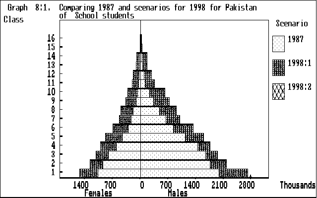
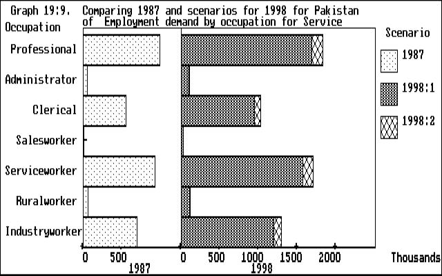
An approach that followed a heuristic approach is the MACBETH model, that will be described in Chapter IV. The results are presented in graphical form allowing a dialogue to be maintained with even the most numerically illiterate policy maker. The system is easy to use and to develop and relatively inexperienced professionals can be quickly trained to use the system. The system is heuristic because it produces results quickly, provokes discussion on the results emanating from the scenarios and leads the inquisitive into the search for new data sources, and better ways of understanding the labour market. The system can be used as a simple tool for continually monitoring what is happening in the labour market.
The MACBETH system was based on this author's idea and first applied to Ecuador by this author with Luis Crouch and Scott-Moreland (Hopkins, 1986). The system applied in Ecuador had a number of weaknesses. These largely stemmed from the short amount of time (three months) spent on data collection, estimation and modelling. Other than the data weaknesses reported upon in Hopkins, the model lacked a complete specification of labour demand it simply used projected output levels and multiplied them by projected productivity levels to obtain projected employment. Further, output growth was exogoneous to the model. These two weaknesses, therefore, did not help to greatly advance the MRA approach. Additions, not tried in the Ecuador model and that have mitigated these weaknesses a little, are described more fully in Chapter IV. In a nutshell the two main improvments have been first, to link output growth to investment and second, to introduce substitution mechanisms so that labour demand is more responsive to market mechanisms.
6. Key informants
Large scale statistical systems with regular (monthly or quarterly) surveys of labour market phenomena are essential for LMIS's. Except in a very few rich countries such systems hardly exist in the world and this is particularly so for the developing world. Richter (1982) has suggested an innovative scheme to provide labour market information through the use of key informants. The idea is to collect selected communitylevel data through key informants using the local knowledge of particular categories of respondents public officials, teachers, businessmen, large farmers etc. This is much simpler and cheaper than a household survey and vastly cheaper than a census. Once reliable key informants have been identified the informants are questioned on a panel basis. The information includes both generalpurpose questions about the overall situation and longerterm trends of labour markets plus specific questions related to shortterm movements and fluctuations in labour supply and demand.
The system has been tested in a number of countries [India, Malaysia, Sri Lanka among others see ILO (1982)]. The overriding conclusion to these tests, unsurprisingly, was that key informant's information was found to be more or less reliable on community level variables such as village characteristics, the problems preventing or impeding the growth of employment like the lack of finance or energy supplies or inadequate transport. It was found to be less good on statistical items concerning the size of the population or the labour force or manpower surpluses and shortages. For most items there was a positive relationship between the quality of the data supplied and the education, age and working experience of the key informants.
In reviewing this experience, Rodgers (1985a) noted five major objections. First, there is a major problem of bias in the selection of respondents since these tend to come from the richer better educated strata of the population. It is likely, therefore, that these key informants will give insufficient stress to the problems of the less rich community and the needs of the poor.
Second, the questions asked tended to be rather simple yet they were addressed to rather complex problems e.g. Is there underemployment? was a typical question and is subject to rather obvious criticisms. Clearly better questions can be formulated and this is not such a major objection to the principle of key informants.
Third, one objective of key informants is rapid feedback to local policy decisions. However, the broad problems raised skill shortage, unemployment etc. are not capable of being entirely dealt with at the local level. They are partly, if not mainly, problems of the macroeconomy. On the other hand Central Governments would be interested in the broad problems raised and, therein, lies another danger. That Central Governments would act on the basis of incomplete, partial and incorrect assessments. Further, local assessments are not likely to be randomly representative and the likelihood of considerable statistical bias could seriously mislead policy makers.
Fourth, the key informant approach is likely to work when the labour market is fairly closed, and thus small enough that individuals can encompass it. This may work in relatively isolated villages, but cannot be easily applied in large urban areas nor where there is close interaction between a village and a large market (e.g. a village on the periphery of an urban zone).
Fifth, as a local system for challenging problems to higher level authority, the key informants system is probably redundant. This is because local elected officials, key businessmen or government employees are in constant contact with the elites of their regions, from which they often themselves come. Emphasizing these channels through key informants therefore seems to be redundant.
In conclusion it would appear that key informants are of limited usefulness to the LMIS. There is not much doubt that random sample household surveys are a cheaper and more robust alternative to censuses. The literature on surveys is burdgeoning (again Rodgers discusses some of these) and there are quicker and cheaper ways of collecting and processing survey information - but see Chapter VII where a key informants survey is reported upon and its advantages and limitations discussed in a practical situation.
7. Labor market signaling
For short-term assessment of training needs labor market signaling (LMS) is recommended as a tool that could both help, and improve, training centers' ability to respond quickly to changes in market circumstances and, thereby, reduce inefficiencies(see Middleton,1993).
"Labor market signaling requires planners to focus on education and training qualifications rather than on occupational classifications. The reasons relate to the quality of occupational statistics, the effect of technology on the concept of an occupation, and the practical link between academic specialization and occupational placements." (Middleton, 1993, p. 140)
This quote of is important because it underlines the basic theoretical model of the World Bank, and most international agencies who tend to take World Bank pronouncements as the status quo. Particularly revealing is the emphasis on education and training qualifications rather than occupations. However, nowhere in the Bank work is a list of skills defined that can be used as a basis for analysis. This lacuna means that no real alternative to an occupational classification has been suggested. Obviously, a fixed occupational classification over the years will ignore technological changes, however there is no reason why these can not be factored in - this is what the most advanced country, the USA, does in practice.
Nevertheless, labor market signaling is a useful adjunct to traditional forms of manpower analysis in that it advocates the need for wage and employment trends not only to guide schooling and training decisions but also to evaluate how well labor markets are functioning. The objective of signaling, again according to Middleton et.al., is that it can estimate whether there will be upward or downward pressure on the economic returns to investment in specific skills. Planners can monitor labor market conditions and evaluate training programs and can also focus upon skills that are of strategic importance to economic development and that take a long time to acquire.
The main indicators or labor market signals required are: wages, employment trends by education and training and occupational classifications, costs of specific education and training programs, enrolment data for institutions, programs of study, individual courses, 'help-wanted' advertisements in newspapers and professional journals, unemployment rates by education, skill, training, occupation.
Part and parcel of the labor market signaling technique is the need to identify the types of skills that are required in the labor market. It is felt that the demand for occupations is a poor predictor of future labor market requirements for qualified labor, simply because the types of occupation change rapidly with new technologies. However, any forecasting technique can compensate through the use of scenario analysis i.e. providing a number of alternative forecasts under different assumptions.
Closely linked to the question of labour market signalling is how to define training needs of a given economy. A first approximation to defining training needs (i.e. skill needs) is to use a list of occupations and then to see whether commonalities in skills can be identified among the occupations. An international standard exists for this and has been developed by the ILO - the most recent being ISCO88 (International Standard for the Classification of Occupations). The main problem with these lists is that they go out of date rapidly as new occupations develop (web designers) and older ones decline (steam engine drivers, punch card operators).
One often hears that training needs cannot be assessed and therefore the best bet is to go and talk to a few enterprises to see what they want. This begs the question of which enterprises, what questions to ask them and how to classify their responses. It also assumes that enterprises know exactly the sorts of occupations that will be in demand after a gestation period of 3 to 5 years - the time taken to place information gleaned from enterprises to policy makers who then determine the types of courses to run in training schools and for this to be put into practice through training teachers, attracting and then training students. In fact the simple-minded statement posed at the beginning of this paragraph summarizes exactly what enterprise surveys of training needs try and establish (see Chapter VII), and what labour market signalling tries to put into practice. We should also note that enterprises work in their own best interests and tend to have a very short-term perspective. Therefore, information collected about enterprises perspectives need to be supplemented with other information. A tracer survey of graduates helps to assess the efficiency of the training school and also to estimate the placement of graduates in jobs. This sort of survey (again see Chapter VII) is very difficult and expensive to carry out but is an effective way of judging the efficiency of training school courses to meet the training needs of the society. Another way to introduce more qualitative and perhaps speculative ideas on the future development of training needs is to ask the practitioners themselves, through a key informants survey as mentioned above.
8. Labour accounting matrices (LAM's)
Grootaert (1986) describes in some detail how to build up a LAM and in his matrix one component of a LAM is that showing headcounts and/or hours worked. In the rows are given 'Types of Individuals' and these correspond to the population and labour supply. 'Types of Individuals' can be disaggregated into In the labour force/out of labour force, each further divided into sex, education and age group. The total, of course, sums to the total population of the nation. Clearly it could be further disaggregated into urban/rural areas.
Next, households are grouped in columns under 'Types of Households' to allow the construction of socioeconomic groups that have relevance with respect to economic and social policy issues. There is quite a range of criteria to describe households and to group them. For some purposes characteristics of the household as a unit are appropriate, such as race or ethnic background, ownership of productive inputs, income level, household size and composition, dependency condition of the household etc. As an alternative, or jointly with household characteristics, some features of the household head or main income earner can be used to describe the household, viz. sex, educational attainment, occupation, industry, employment status, earnings etc. Most censuses will allow the construction of such a block.
The second building block describes the basic economic status of the individual members of the population. Under the heading 'Productive Activities' a first major dividing line could be whether or not an activity results in economic output, i.e. contributes to GDP according to the UN definition. It is possible, of course, to deviate from the UN guidelines to include all nonmarket activities the UN only includes selected nonmarket activities. This could then be subdivided into a classification scheme such as the ISIC scheme, then further subdivided into formal/nonformal activities and/or public/private. Individuals could also be distinguished by the number of hours they work or some other definition of employed/underemployed. To turn the LAM into a manpower matrix individuals could be further divided into educational or occupational categories. The LAM is then a manpower matrix because it indicates the number (or number of hours) that each type of person is, on the average, available for work. The matrix of activities can either be a supply or a demand for labour statement and shows the numbers each type of individual spends being engaged in productive activities and the number of hours that are lost due to unemployment.
'Other activities' could include unemployment, nonmarket activities, schooling, retirement, homemaking etc. These could be relocated under the heading of 'productive activities' should it be so desired. Note that the left hand side of the matrix 'Types of Individuals' provides a number of difficulties for the allocations in 'Productive (or Other) Activities'. For example, identifying those in the informal sector is difficult enough without the added complication of age/sex disaggregations.
Under 'productive activities' the seasonality dimension could be added to the labour force matrices. It could be available as both a head count table and a table with number of hours, this set of tables would permit the analysis of the seasonal pattern of job availability. It could indicate which type of jobs open up during which season, and how many hours of work they provide and which types of individuals (age/sex/education) obtain all year round jobs versus seasonal jobs. It could give information about hours of work during peak and slack seasons which is useful to estimate the opportunity cost of time.
In order to examine the relations between economic variables and the LAM we might wish to link our LAM into a SAM. To do this we need to add a number of other items to the matrix. The remaining factors of production, land and capital goods need to be introduced. Since these factors are not only owned by households, but also by firms and by the government, columns for these institutions need to be added to the accounting scheme. Again the accounting can be accomplished in headcount, hours worked or value. To complete a LAM to a full SAM, links with the rest of the world, transfers within and across institutions, demand for commodities, an inputoutput table and current and capital accounts must be added. An example of an application of a LAM in Kenya can be found in Vandemoortele (1986). He describes how, using a SAM in a comparative statics framework, an exogoneous change in the distribution of income can be shown to affect employment and output. Since a LAM is a subset of a SAM the model also applies toLAM's.
The first step in developing a SAMmodel is to separate the endogoneous accounts from the exogoneous ones so that the impact of the latter on the former can be measured. The endogenous accounts generally comprise the factor accounts, the accounts for households and companies (the endogoneous institutions) and the accounts for the production activities. The exogoneous accounts include the government account, the investment account, the accounts for indirect taxes and international transactions. The classification is set out in Figure 1 below.
 Fig1(i): Exogoneous and endogoneous submatrices
Source: Vandemoortele (1986) based on Pyatt and Roe et.al.(1977).
Fig1(i): Exogoneous and endogoneous submatrices
Source: Vandemoortele (1986) based on Pyatt and Roe et.al.(1977).
The northwest submatrix constitutes the matrix of transactions between the endogoneous accounts, and the southeast submatrix is the transaction matrix of the exogoneous accounts. The northeast submatrix is the injection matrix while the southwest submatrix is the matrix of leakages. The accounts are normalised, just like inputoutput analysis, by dividing the matrix elements by the column totals. The application of LAMs to the manpower planning problem is not widespread probably because of the use of fixed coefficients so that the allocation of labour by economic sector, for instance, is carried out in the same way as the discarded manpower planning approach. In fact the LAM is simply a formalisation of the data from a manpower planning exercise into a set of accounts. This is useful in itself as a way of organising data but still does not escape the aforementioned limitations.
9. Concluding remarks
The chapter has covered the main manpower planning techniques - manpower requirements, rate of return, labour market information systems, pragmatic, key informants, labour market signalling and LAMs. There are, of course, overlaps between each of the techniques suggested but none of the approaches has come to dominate in practice. Despite the lack of consensus on technique to be used, the demand for manpower projections runs unabated. Indeed, the Bureau of Labor Statistics (BLS) 3 in the USA uses a combination of MRA and economic forecasting while the author has recently completed a manpower analysis for the Asian Development Bank (ADB) in Vietnam where the authorities were keen to know the future demands for skilled manpower in their economy to revamp their vocational education system. This experience is described in the last chapter where it can be seen that a mixture of most of the techniques described in this chapter were used depending on the precise question addressed.
References
- B.Ahamad and M.Blaug (eds.): The Practice of Manpower Forecasting:A Collection of Case Studies, (Elsevier, Amsterdam, 1973).
- J. Behrman and A. Deolialikar: "Are there differential returns to schooling by gender? The case of Indonesian Labour Markets", Oxford Bulletin of Economics and Statistics, 57, 1 (1995), 0305-9049
- P. Bennell (1996a): "General versus Vocational Secondary Education in Developing Countries: A Review of the Rates of Return Evidence", Journal of Development Studies (Frank Cass, London), Vol. 33, No. 2., Dec 1996, pp230-247
- P. Bennell (1996b): "Using and Abusing Rates of Return: A Critique of the World Bank=s 1995 Education Sector Review", Int. J. Educational Development, Vol. 16, No.3, pp.235-248, 1996 (Elsevier, 1996)
- M. Blaug: Economics of Education (Penguin, 1970, Harmondsworth, UK).
- C.Colclough: 'Why has the manpower planning debate not yet been resolved?' mimeographed, IDS, University of Sussex, Working Paper, July 1987.
- S.Cole et .al.: Global Simulation Models (John Wiley Sons, London, 1975)
- L.Crouch and R.ScottMoreland: 'Manpower supply as an output of the educational system', Research Triangle Institute , Working Paper (January, 1987).
- J.Defourney, E.Thorbecke: 'Structural path analysis and multiplier decomposition within a Social Accounting Matrix Framework', in Economic Journal (London), March, 1984, 94(373), pp.11136.
- C.R.S. Dougherty: "The optimal allocation of investment in education", 1971, in Chenery, H. ed., Studies in Development Planning (Harvard University Press)
- C.R.S. Dougherty: 'Manpower forecasting and manpowerdevelopment planning in the United Kingdom', in R.V.Youdi and K.Hinchliffe (1985, op.cit.)
- C.Grootaert: 'The Labor Market and Social Accounting:A Framework of Data Presentation' (World Bank, LSMS Working Paper No.17, 1986).
- A. Hazlewood: Education, work and pay in East Africa, (Clarendon Press, Oxford, 1989)
- R.G. Hollister: 'Manpower Planning Viewed as an Analysis Process for Manpower and Employment Policy Formation and Monitoring', (Mimeo, Swarthmore College, USA, 1986)
- M.J.D.Hopkins, L.Crouch, R.ScottMoreland: 'MACBETH: A Model for Forecasting Population, Education, Manpower, Employment, Underemployment and Unemployment', (ILO Working Paper, WEP 243/WP. 11, Geneva, September, 1986).
- J. R. Hough: "Educational Cost-Benefit Analysis", ODA, Education Research, Serial No.2, undated.
- ILO: Labour Market Information through Key Informants (Geneva,1982).
- ILO: Employment Planning (PREALC, Santiago, 1984)
- R.Jolly and C.Colclough: 'African Manpower Plans: An Evaluation', in International Labour Review (Geneva), AugSept., Vol. 106, Nos 23, 1972.
- B.B.King: 'What is a SAM? A layman's guide to Social Accounting Matrices' World Bank, Staff Working paper No.463, Washington, 1981.
- J. Lauglo: "Banking on Education and the Uses of Research A Critique of: World Bank Priorities and Strategies for Education", Int. J. Educational Development, Vol. 16, No.3, pp.221-233, 1996 (Elsevier, 1996)
- Sanjaya Lall: "Competing with Labour - Skills and Competitiveness in Developing Countries", Issues in Development, Discussion paper 31 (POL/DEV, ILO, Geneva, Aug., 1999)
- W. Mason: Guidelines for the development of employment and manpower information programmes in developing countries : A practical guide (ILO, Geneva,1979)
- S. McGrath and K. King with F. Leach and R. Carr-Hill: "Education and Training for the Informal Sector", Education Research, ODA, Vol. I, March 1995
- John Middleton, Adrian Ziderman, A. Van Adams: Skills for Productivity - Vocational Education and Training in Developing Countries, Published for the World bank by Oxford University Press, New York, June 1993. See also MOE-GTZ: "Skills Training Needs Analysis Survey", Lao PDR, 12 Nov 98; MOLISA (CEPRH/ORSTOM): "Observatory System of Employment and Human Resources in Vietnam", Hanoi, 1998.
- J. Mincer: "Schooling Experience and Earnings", (National Bureau of Economic Research/Columbia University Press, New York).
- C. de Moura-Castro: 'In defence of planning (but only up to a point', in International Labour Review, (Vol. 130, 1991, No.4).
- H. Parnes: Forecasting educational needs for economic and social development, Paris, OECD, 1962
- F.Paukert, J.Skolka, J.Maton: Income distribution, structure of economy and employment (London, Croom Helm, 1981).
- G.Psacharopoulos: 'Indonesia: Manpower Considerations in the Energy Sector and Elsewhere', Interim Report, mimeographed, C89898/J87843/D2620/02, (World Bank, Washington, Dec, 1981).
- G. Psacharopoulos: 'From manpower planning to labour market analysis', in International Labour Review, (Vol. 130, 1991, No. 4).
- G. Psacharopoulos: "The Profitability of Investment in Education: Concepts and Methods", Human Capital Development and Operations Policy, Working Papers, Nov. 1995, (The World Bank, Washington, DC)
- G. Psacharopoulos (1996a): "Building Human Capital for Better Lives", Feb. 1996, (The World Bank, Washington, DC)
- G. Psacharopoulos (1996b): "Designing Educational Policy: A Mini-Primer on Values, Theories and Tools", Int. J. Educational Development, Vol. 16, No.3, pp.277-279, 1996 (Elsevier, 1996)
- K. R. Popper: Conjectures and Refutations: The Growth of Scientific Knowledge (Routledge and Kegan Paul, London, 1963)
- G.Pyatt and A.Roe and associates: Social accounting for development planning (ILO, Geneva, 1977).
- G.Pyatt and E.Thorbecke: Planning techniques for a better future (Geneva, ILO, 1976).
- Research Triangle Institute, 'The HOST modelling system a computer program for microcomputers', USAID, available free from RTI, Research Triangle Park, North Carolina, 1987.
- P. Richards: 'Issues in Manpower Analysis', in New Approaches to Manpower Planing Analysis, P.Richards & R. Amjad (eds.), (ILO, Geneva, 1994).
- L. Richter: 'Manpower and Employment Information through Key Informants', International Labour Review (Geneva), MayJune 1982, Vol.121, No.4, pp417431.
- L. Richter: 'Upgrading Labour Market Information in developing countries: Problems, progress and prospects', (ILO, Geneva, 1989)
- G.B.Rodgers, M.Hopkins, R.Wery: BACHUEPhilippinesPopulation, Employment and Inequality (Saxon House, U.K., 1978).
- G.B.Rodgers: ' Labour Market Information: Issues, Users, Key Informants and Household Surveys' (Mimeo, ILO, Geneva, August, 1985a)
- G.B. Rodgers: 'Labour markets, Labour Processes and Economic Development : Some Research Issues' ,(WEP Working Paper, ILO, Geneva, Sept. 1985b) - crossed out first reference!!
- S. Sigurdsson and E. Schweitzer: "Performance Indicators in Bank-Financed Education Operations", Second Edition, Human Development Department, Dec., 1995 (The World Bank, Washington, DC)
- SPSSinc.: Data entry: SPSS/PC+ for the IBM PC/XT/AT (SPSSinc., Chicago, Illinois, 1987).
- Bertrand Russell: In Praise of Idleness (London, George Allen and Unwin, 1976).
- G.Standing: Labour force participation and development (Geneva, ILO, 2nd ed., 1981).
- G.Standing and G.Sheehan: Labour Force participation in lowincome countries (ILO, Geneva, 1978).
- United Nations: 'Manual On Integrating Population Variables into Development Planning', Ad Hoc Expert Group Meeting, ESA/P/WP/87, (UN, New York, 1985).
- J.Vandemoortele: 'Socioeconomic analysis and planning within a social accounting framework', (ILO, World Employment Programme, Working Paper, WEP 243/WP.5, June 1986).
- R.Van Der Hoeven: Planning for Basic Needs : A Modelling Approach , (Gower, London, 1988).
- World Bank: 'Tunisia Industrial Employment' (Washington, EMENA, Country Programs Dept.II, March 1985).
- R.V. Youdi and K.Hinchliffe (eds.): Forecasting Skilled Manpower Needs: The Experience of eleven countries , (UNESCO, Comedi, Belgium, 1985).
II: An overview of major theories of labour market mismatch 4
1. Introduction
Manpower planning has, at its core, the problem of mismatch between labour supply and demand i.e. unemployment. Consequently, a better understanding of the manpower planning problem can be helped by examining theories about the determination of unemployment. Therefore, this chapter overviews some of the leading strands of thought that have attempted to explain, among other things, the economic causes of unemployment. This is an ambitious undertaking since the field is vast and, therefore, the approach taken has been eclectic and does not pretend to be exhaustive. The main choice has been to include those theories, and theoreticians, that have focussed upon unemployment rather than economic theory per se. So, Marx, Keynes and Lewis are included while, for instance, Sen, who focussed mainly on poverty and entitlements, Myrdal, of Asian Drama fame, and Tinbergen, who focussed upon CGE models, are not. Moreover, the discourse has been hampered because economists rarely agree among themselves on what is the most appropriate theory. For example, in a discussion on the Nobel prize winners for economics, Little 5 stated:
" Clearly, Lewis got it for stating that the marginal product of agricultural labour is zero, and Schulz for showing that it is not"!
Most theories do not centre on the causes of unemployment 6 ; rather they are mainly concerned with what causes, inter alia, accumulation, changes in the profit rate, inflation, growth, or changes in wages. Clearly, these causes are interrelated and so the emphasis of theory on a number of problems at once is not altogether surprising. The word 'overview' has been used since it is difficult, if not impossible, to describe adequately all theories, thus the chapter's main purpose is to identify what the different theories say about the causes of unemployment as a forerunner to the presentation of a simulation model of the labour market in later chapters.
Theories have been considered that apply both to developing and to developed countries because, while countries at different stages of development have different settings for their common problems, theory transcends these boundaries. However, this should not imply that there is, or ever will be, a unique theory that can be applied everywhere or at different stages of development. As Kornai 7 has remarked, there is no such thing as an optimal system containing the best possible rules. Planning an economic system is not like visiting a supermarket where on the shelves can be found the various components of the mechanism incorporating the advantageous qualities of all systems. 'On one shelf there is the high degree of workshop organisation and discipline as in a [Federal] German or Swiss factory. On another there is full employment as it has been (nowadays as was) realised in Eastern Europe. On a third shelf is an equality of income and purpose such as found in Mao's China. On a fourth is economic growth free of recession, on a fifth price stability, etc.' This should not imply that pragmatism is the alternative. Theory can help in setting guidelines and has a perverse affect in entering decision making hence carrying out Lord Keynes' dictum that present day policy makers, unbeknown to them, are carrying out the theories of some defunct economist!
In this chapter theories dealing with the labour market will be discussed in temporal order. They have been arranged into seven main groups in order to preserve some common factors, namely classical theories (Smith, Ricardo, Malthus, Mill, Marx); neo-classical (Say, Marshall, Schumpeter, Pigou, Hayek, Wicksell, Walras, Solow, Harrod, Domar, Schultz, Stiglitz); social reformers (Keynes, Lenin, Kornai); latter-day development economists (Lewis, Fei, Ranis, Prebisch, Hirschman); monetarists (Friedman); more recent development economists who are institutionalist in persuasion such as the segmentation theorists (Carnoy, Harris, Todaro); and, finally, recent views of the labour market (Krugman, Fine). In this list there are gaps and overlaps between the different schools. Many would say that there exist today, at the most, two main schools of theory: neo-classical and non-neo-classical or institutionalist. But this is an oversimplification, because there are theories or ideas from one school that can be applied in the other. For example, at different times Keynes could have been considered a classical, neoclassical, Marxist or even monetarist scholar since there are strands of each school in his writings.
2. Classical economists
These economists, working in the mid-nineteenth century, were greatly concerned with the interactions between labour, capital and land. Adam Smith in The Wealth of Nations, first published in 1776, was concerned with the principles of free competition and the 'invisible hand' of the open market. Few economists would disagree with Smith that markets work when one important condition holds namely, actors in the market have equal weight in terms of size of firm, information, human and physical capital. Imperfections or unbalances in these initial conditions in the real world have lead to the enormous and burgeoning economic literature of today and the attempts to resolve these overriding qualifications have led to the growth of economics as a science.
For Smith 8 , the growth of the labour force was related, on the supply side, to population. In the long run he believed that population growth was regulated by the funds available for human sustenance. Consequently, the wage rate plays a crucial role in determining population size. The limiting wage was that which was neither sufficiently high to permit an increase in numbers, nor sufficiently low to force a shrinkage of the population base. Smith called this rate 'the subsistence wage', one which is consistent with a constant population. Smith argued that in a purely competitive market, if the wage rate fell temporarily below what was necessary to maintain labour demand and supply in balance, the pressure of demand would act to raise it. Conversely, should wages be above the equilibrium level, then the excess supply resulting from too rapid a growth of population would soon lower the remuneration of labour. But what determines the demand for labour? In Smith's words 9 , 'the demand for those who live by wages, it is evident, cannot increase but in proportion to the increase of the funds which are destined for the payment of wages. These funds are of two kinds: first the revenue which is over and above what is necessary for maintenance; and, secondly the stock which is over and above what is necessary for the employment of their masters.' This is the wage-fund doctrine. It relates the employment of labour to the size of the revolving fund destined for the maintenance of the labour force.
An illustration of Smith's view, following Samuelson 10 , is given in figure 1.
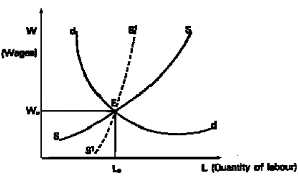 Fig1(ii): Demand and supply curves for labour
The demand and supply curves for labour intersect at full employment E, at a wage of WO and a quantity of labour LO i.e. labour will offer itself either at an equilibrium wage level or, if there is excess demand for jobs in the system, workers will reduce the wage at which they offer themselves until equilibrium is reached. (The dotted line S1S1 indicates a more inelastic labour supply function.)
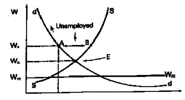 Fig2(ii): Unemployment and competitive wage cuts
Fig2 11 illustrates how Malthus' theory of population implies a constantly increasing supply of labour at subsistence level Wm at which people will just reproduce their numbers. Both Adam Smith followers and Keynesians disagreed with Malthus. The former because prices would adjust through the magical hand of the market and people would change their behaviour after seeing that the production of children led to their impoverishment. The latter because Malthus' theory ignored the Keynesian demand effects of a growing population 12 which would serve to push up incomes and the level of living above subsistence level. Today, as environmentalists vigorously argue for the reduction of the use of non-renewable resources, Malthus has again come back into fashion.
Marx's 'reserve army of the unemployed' - as shown by AB in Figure 2 - need not depress real wages from Wx to the mm minimum subsistence level. With perfect competition it can only depress wages from A to E. If labour supply became so abundant that SS intersected dd at mm, the wage would be at a minimum level, as in many underdeveloped regions. But institutional or legal changes can do little when marginal productivity is so low. That open unemployment has remained around the 10-20 per cent level in many developing nations over the past 20 to 30 years suggests that these simplistic diagrams cannot totally be relied upon. This is discussed later in the section on segmented labour markets (SLMs).
David Ricardo, as a forerunner of Marx, focussed his studies upon the distribution of the social product and, according to Hagen 13 , established two main principles. One was that wages could only increase with rises in the accumulation of capital. The second principle was that the landowning class contributed a growing social weight whose power could be reduced only through free imports of agricultural products.
Ricardo's production function, like Adam Smith's, postulated the existence of three factors - land, capital and labour. In contrast to Smith's function, however, Ricardo's was subjected to diminishing marginal productivity 14 , which stems from the fact that land is variable in quality and fixed in supply. As a result the marginal productivity not only of land itself but also of capital and labour, declines as cultivation is increased. As many have remarked, a great weakness here is that Ricardo underrated the possibility of technological advance in agriculture. Ricardo's notion of population and labour supply was similar to that of Smith, except that he believed that, because of capital accumulation, the market wage could rise above subsistence level. Yet, if labour supply exceeded labour demand, the market wage would fall to subsistence level so that labour demand would eventually equal supply.
Karl Marx's provided the first major critique of capitalism based upon his observations of the labour market in nineteenth - century England. According to Furtado 15 , the force of Marx's vision was concentrated on two main things: first, identification of the fundamental relation of production of the capitalist mode, and second, the determination of the major influences that develop the factors of production. Marx identified two main classes - capitalists and workers - and believed that the owners of capital would always seek to maximise profit (or surplus value as he called it) while paying workers a subsistence wage. These wages would allow labour to reproduce itself in order to maintain a reserve army of unemployed. Capitalists could, therefore dictate both employment and wage levels.
To analyse capitalism, Marx introduced the labour theory of value. Simply, this means that if 1 kg of rice were to be produced by 1 labourer in 1 week, and 2 kg of flour by 1 labourer in 1 week, then l/2 kg of rice should have the same value as 1 kg of flour. Marx defined surplus value as the unpaid work of the workers. The total product of nation, called the social product (P) was equal to the sum of constant capital (C) [depreciation, raw materials used in production, and energy inputs], variable capital (V) [paid salaries] and surplus value (M), i.e.
P = C + V + M ... (1).
Marx defined the rate of exploitation of the workers as M/V, C/(C+V) as the index of organic capital needed to create new value, and M/(C+V) as the profit rate. For accumulation, only surplus value could be transformed into capital (equivalent to the classical assumption that Investment = Savings). Marx did not indicate clearly what principles governed the distribution of surplus value between consumption and accumulation by the capitalist class. Considering that each capitalist simply struggled to increase surplus value, Marx did not much care about the conflicts within the capitalist class.
Marx predicted the demise of capitalism 16 within the next 10 to l00 years, through a 'crisis'. This would come about because the capitalist mode of production produced a progressive relative decrease of variable capital as compared to constant capital so leading to a progressive fall in the rate of profit. This would lead, from equation (1) above, to a reduction in surplus value and hence reduction in the accumulation of capital. This process continues until capitalism collapses because of massive unemployment and social unrest. Capitalists could try and prevent this by (a) more intense exploitation of the workers through reducing wages, (b) exporting capital to the colonies, (c) swelling accumulation in order to raise the quantity of profit. For the 'crisis' to occur, there would have to be persistent insufficiency in effective demand. A number of 'crises' have indeed occurred in capitalist economies over the past 100 years. These have been characterised by a sharp increase in unemployment coupled with a slow-down or reduction in production. To date, governments in industrialised countries have bought their way out of crises through two main measures: deficit financing, more often than not forced upon them through wars and through social security payments to the unemployed. Hence Marx's crisis of capitalism has been avoided through positive Government intervention on behalf of the workers and thus changed the relation between the accumulation of capital and unemployment.
In the United Kingdom - Marx's nineteenth-century model - the major depression of the 1930s was finally resolved as war intervened, stepping up public works and preventing another crisis. The war was followed by an intensive social security effort to compensate workers in unemployment. The labour movement in the United Kingdom steadily increased its power but channelled its major efforts into the formation of a political party - the Labour Party - which was elected into office for the first time in the 1930s. The introduction of benefits for workers has propped up the British economy and dampened social unrest up to the present day.
Marxist theories provided an essential and useful critique of capitalism. The ideas of Marx were taken up by Lenin and gave the world Marxist-Leninist thought. This was applied in Eastern European countries under Soviet leadership, all of which were successful in providing full employment. However two main aspects eventually led to its demise. First the standard of living remained low compared with Western economies and second, a high degree of repression of human rights was required to preserve the command economy.
3. Neo-classical economists
These theories underline the importance of market forces in bringing systems into equilibrium. Their main addendum to classical economic theory is their focus on the regulatory role of prices, i.e. they differ with economists such as Smith only in terms of emphasis. That markets for goods or labour do not clear, they believe, is a matter of distortions in the price system. Unemployment occurs because the price of labour (wages) relative to the price of capital (interest rate) is too high. If labour reduces its price it will be absorbed.
This view can be attributed to any number of economists but perhaps Marshall was the forerunner. This area is rich in mathematical models, the most typical being that of Walras 17 which has two factors of production (capital and labour), two commodities and two production functions characterised by Leontief style fixed coefficients. All product markets are cleared through price adjustments to a 'Walrasian equilibrium'; the model therefore assumes full employment. There is no mechanism to introduce demand. In a dynamic version of this model, the Harrod-Domar model 18 , Y = K/u (Y = output, K = capital, u = constant capital output ratio), u is fixed and hence the economic system is geared to a steady state of growth. In this model there is no market mechanism to equilibrate demand and supply of labour, hence the rate of growth of production may well be exceeded by the exogoneously determined rate of growth of the (working) population. The result could be an exponential unemployment growth rate. Solow 19 rescued this model from positing the inevitability of unemployment by arguing that the choice of technique, the capital- output ratio, could shift in response to a growing availability of labour, as could the savings ratio. Labour could be absorbed if the 'technique' was right since, over time, the price of labour would dictate the technique. This was perhaps the birth of the idea of labour intensive techniques where it is suggested that labour can be absorbed for a given output by choosing an appropriate technique. Presumably if market pricing were working, such a labour intensive policy prescription would be unnecessary. This is because if, in a neo-classical world, the price of labour is attractive to producers compared to the price of capital, labour will be absorbed through an appropriate choice of technique. If labour is not absorbed, it implies that there are other factors at work. This is a phenomenon that has been observed recently in industrialised countries. The fight against inflation has been led by increases in real rates of interest. This has made the price of capital dear compared with labour, yet the result of the policy has been reduced inflation but higher, not lower, unemployment since high interest rates have prevented investment and growth and, consequently, this has led to the shedding of labour. As real interest rates reduced, borrowing and therefore investment costs reduced promoting increased economic growth. This led to greater rates of labour absorption, at least in the UK and USA where unemployment rates have fallen significantly in the 1990s. In Europe, unemployment has fallen but remained high due, it is argued, to institutional factors. What these other factors are that have prevented the absorption of labour can be found in examining institutional barriers to the setting of wage rates and in the discussion of dependency theories suggested by Prebisch when working in ECLA. His theory is summarised in section 5 below as is the contemporary debate between the World Bank neo-classical economists and the ILO institutionalists.
In a later article Solow 20 , turning away from his earlier stance, has admitted the existence of institutional factors in explaining unemployment. He asked whether one should think of the labour market as mostly clearing, or at worst, in the process of a quick return to market-clearing equilibrium. Or should one think of it as mostly in disequilibrium, with transactions habitually taking place at non-market clearing wages? Solow sides with the latter, quoting the more recent work of the classical economist, Pigou 21 . In that work Pigou finds four main reasons why the labour market does not operate as if workers were engaged in thoroughgoing competition. First, because the labour market is segmented C e.g. unemployed, unskilled labourers cannot compete for jobs held by craftsmen. Second, trade unionism and wage stickiness restricts movements to equilibrium wages. Third, the provision of unemployment insurance has made workers more resistant to accepting employment even when wages are above unemployment insurance (why work for 20 per cent more than unemployment benefit when this can be replaced by leisure or informal sector earnings ?). Fourth, workers know the rate for the job and are reluctant to accept less than the going market rate. In his presidential address to the American Economic Association, Solow asked his audience whether they themselves would not be surprised if they learned that someone of roughly their status in the profession, but teaching in a less desirable department, had written to their department chairperson to teach their courses for less money. Clearly this does not happen.
The great challenge to classical and most neo-classical ideas, at that time, and the inevitability of unemployment, came from Lord Keynes 22 . As Klein 23 argued, and Keynes himself stated 24 , Keynes theories were a reaction to the classical economists. For example, one of the main classical theories was put forward by Say, and known as Say's law, which in its popular form claimed that supply creates its own demand. But Keynes' main source of classical thought was Pigou who, in his earlier work 25 , believed that the 1930 unemployment in the United Kingdom was caused by the improper allocation of people to jobs and the existence of wage rates above the level called for by the general demand conditions. Following these lines of argument, Pigou supported a policy of wage cuts. Schumpeter too, believed that there could be no persistent unemployment in a perfect, frictionless capitalist system. Aside from his theory of innovations which explained relatively short period movements, he claimed that 26 the forces at work in the early period of the 1930 depression were the agrarian crisis, protection, high taxes, interest rates and wages, and the lack of free price movements. Nevertheless, while Schumpeter could see no valid economic reason for the breakdown of capitalism, like Marx before him, he predicted that the capitalist form of society would eventually be superseded by socialism 27 .
More recent neo-classical contributions to the development debate include Schultz' reassertion of the importance of investment in human capital 28 and Stiglitz, Krugman (and others) attempt to found a new development economics on the basis of a theoretical exploration of the nature and implications of the rationality of small-scale producers 29 . These later neo-classical views are discussed in the penultimate section below.
4. Social reformes
Keynes thought that capitalist systems were perfectly viable if it were not for artificial barriers and felt that an unequal distribution of wealth was necessary to maintain the level of savings high enough to supply the abundant demand for capital formation. The principal difference between Keynes and the classicals was in the determination of equilibrium. Keynes argued 30 that the volume of employment in equilibrium depended on (1) the aggregate supply function, (2) the propensity to consume, and (3) the volume of investment. This was the essence of his General Theory of Employment. The classical economists insisted that prices would change to make supply equal demand in product, capital and labour markets. Keynes essentially argued that quantities would change to achieve equilibrium, and that real wages were rigid (actually he did not assume this, but dropped the assumption of perfect information). From the simple Keynesian model given in figure 3 it can be seen that, if there is a fixed quantum of labour and if labour supply is determined by wages, then any decline in aggregate demand (AD) and hence output (Y) produces more unemployment.
 Fig3(ii): Simplified Keynesian model
It can be seen, further, that, if the wage bill is increased (i.e. c increases), profits will be squeezed and savings and investment will drop. This need not occur if foreign capital flows are obtained, if the government runs a deficit or if the government taxes that part of the income of the rich that does not go to savings. Also, a reduction in real wages exacerbates the situation since it reduces aggregate demand. All these follow from the Keynesian model. As Klein 31 remarked, full employment in socialist countries follows directly from Keynes since any sensible central planning board will set the amount of investment at a level which would just offset savings out of a full employment national income. It was once thought by some Marxist economists, such as Paul Sweezy of the United States, that the class-based division inherent in government will not allow the liberal social reform required by Keynesian economics 32 . The convergence between Marxists and Keynesians is strong in neo-Keynesian economics where vigorous government intervention is suggested to achieve full employment. And both economic schools agreed 33 that capitalism faces the problem of aggregate demand C that is, will the level of aggregate demand generated by any level of output be sufficient to purchase the whole of that output?
Implementation of a Keynesian approach requires an activist government to achieve full employment. As Bhatt 34 remarked, how can governments assume responsibility for the maintenance of adequate investment growth without inquiring further into the pattern of investment which is so relevant to the nature and structure of growth and welfare?
In developing countries a Keynesian approach suffers from a number of problems. Berry and Sabot 35 have pointed out three of these. First (following Reddaway 36 ), although there is abundant labour, at least of unskilled types in the poorer nations, a general increase in demand will not lead to a general increase in output, because other co-operating factors are needed to work with labour. The traditional one to take is capital, i.e. real capital equipment, 'nothing much can be done with bare hands alone'. The MACBETH model, described in Chapter IV and applied to Sri Lanka in Chapter V, illustrates this as increased aggregate demand leads to increased demand for educated labour but overall unemployment remains high since uneducated labour cannot be absorbed with the technological mix chosen. Adrian Wood has also modelled this in his two sector, two country model of trade and comes to the same conclusion 37 .
Second, demand deficiency tends to ignore longer-run influences on output such as the negative effects of population growth, and the positive effects of technological change and capital accumulation. Technological change is more difficult to quantify; new techniques can be introduced at a marginal productivity lower than the wage rate of labour even though a number of institutional factors, such as social investment, quality of product and environment, may make them undesirable. On the other hand entrepreneurs often prefer to buy in technology which is both labour saving and enhances product quality. Labour saving technology is often preferred in developing countries, despite low wages, because of rigid labour legislation that hinders labour flexibility.
Third, the specificity of location and the pattern of unemployment, which, in LDCs, may be urban surplus and rural scarcity, contradict the Keynesian models that maintain that the direction, if not the rate, of change in aggregate demand is the same in all sectors.
The Hungarian economist Kornai's analysis is interesting in that it embodies both neo-Keynesian and Marxist thought. Kornai believed that the inefficiencies in the capitalist mode of production, as exemplified in the West, manifested themselves mainly in terms of unemployment. In the former socialist countries of Eastern Europe, inefficiencies manifested themselves not in unemployment but in the form of shortages 38 . Hence it was not possible to discuss problems of unemployment in centrally planned economies since it simply did not exist. The main problem was that of shortages in the supply of goods both consumed and produced. The absence of incentives or price signals in the system would not allow a rapid response of the forces of production. This was the key economic problem of centrally planned economies. Hungary, under Kornai's persuasion among others, led to the partial re-introduction of competitive markets well before most of the other former Socialist countries. This has given it a head start and is now generally believed to be one of the successes of the transition from socialist to a market economy.
As Kornai remarked, in Hungary the centralisation of economic management started in 1948-49 39 . The majority of firms were nationalised and a wide co-operative sector was established. Public firms were controlled centrally, with the aid of a hierarchical multi-level apparatus. The fulfillment of production plans given to firms, as well as adherence to the input quotas allotted to them, was obligatory. Price setting and the allocation of investment were highly centralised. The main purpose of the 1968 reform was to free public firms from bureaucratic ties and increase their autonomy. The firm did not then receive a binding directive as to what it should produce in the next year and rationing of inputs through fixed quotas almost ceased. Hungary's former 'command economy' was then replaced by a system in which independent firms were connected, to a large extent, through the market. Some prices continued to be set centrally but the number of contract prices determined by the seller and buyer were enlarged considerably. Investment decisions were shared among central organisations, credit-granting banks, and the firms themselves who were able to finance part from their own savings.
The reform brought tangible results, according to Kornai, with production growing at 5-6 per cent yearly during the ten years after the reform. Full employment continued and, in some cases, led to a labour shortage. Real wages rose regularly, the supply to consumers noticeably improved, and the variety of consumer articles widened. However, the pace of change put into place by these reforms accelerated the eventual rejection of centralism and a wider embrace of market mechanisms.
5. Development economists
Development economics is generally thought to be a poor relation to mainstream economics. This is because, it is argued, the developing countries are so poor in natural resources, technology, capital and skilled labour that their problems only require rudimentary analysis. However, Krugman 40 argues that the fading away of development economics, especially post Myrdal, Hirschman and Lewis after the 1960s has been because "the rhetoric of development theory has been to cover poorly conceived or even corrupt policies". These structuralist theories were the orthodoxy of development economist who (apparently) believed that developing country markets are rigid and need to be pushed into action by government (Little 41 ). The new orthodoxy, argued Krugman, was that by 1980 there was a belief in the efficacy of free trade and free markets for developing countries and that its intellectual credibility was "under-pinned by the demonstration of market efficiency in neo-classical general equilibrium theory". Thus this new orthodoxy effectively denies that there is anything special about the situation of developing countries compared with those of developed nations. This point of view was broadly confirmed by two economists at the same conference - Stiglitz and Jayawardena. Although Stiglitz noted 42 that if, as Krugman states, economies of scale are significant then larger economies should be better off and this is patently not so and, second, that technology is less effective in developing countries simply because information is costly to obtain and disseminate. While Jayawardena agreed 43 that none of the ideas spawned by the development literature, such as the "big push", played any essential role in motivating today's development orthodoxy now known as the "Washington consensus" (see below). But the main point of Krugman, albeit self-serving, is that if the earlier development economists had had the economic tools of today then there insights would have fared better.
In the rest of this section, nonetheless, are considered the theories of six economists who were the inspirators of the field of development economics and who have made major contributions to development economics during the thirty years or so after the Second World War, namely Arthur Lewis, Fei, Ranis, Prebisch, Hirschman and Paul Schultz .
Arthur Lewis in his seminal paper 44 characterises developing countries to have an unlimited supply of labour, and with population numerous in relation to capital and natural resources. The marginal productivity of workers in agricultural activities can be negative because, when labour supply is very much greater than demand, there is no need to pay more than subsistence wages even though these are probably less than the average product. According to Lewis, high rates of population growth provide a high rate of growth in labour supply and, consequently, a continuing downward pressure on wages. Lewis' celebrated dualistic model considers two main producing sectors C capitalist, in which capital is reproducible and where capitalists receive a rent from ownership of it, and subsistence, in which reproducible capital is not generally used. Salaries in the capitalist sector are related to those in the subsistence sector, hence capitalists have a direct interest in keeping down subsistence wages. In agricultural sectors the subsistence wage is exogenous to the supply and demand of labour, and unemployment is the result of an economy-wide rigid wage in excess of the market clearing level. For example, a piece of land that can be fully cultivated by two people may actually be worked by four, if four working men in a household have no other employment opportunities and happen to own the land; each of the four would, in effect, work half time but for the same subsistence wage. Thus, in that case, the supply and demand of labour does not influence the subsistence wage.
Alternatively, capitalist sector wages can be 30-100 per cent more than the subsistence wage because of cost-of-living differences (although this is probably illusory because of higher prices in the capitalist sector which tends to be in urban areas). Furthermore, discipline amongst workers, even in the absence of trade unions, means that job applicants refuse to accept lower wages than those existing workers receive - note that this differs from the neo-classical school. Savings and investment increase because most savings come from the rentier class and few from the working class. This is because if there is an unlimited supply of labour at a constant real wage, the capitalist surplus will augment continually and annual investment will be proportional to the growth in national income. This cannot go on for ever since, for example, all labour might be absorbed at subsistence level wages because capital accumulates faster than labour supply. Then wages will rise and profits fall. Hence the capitalist sector cannot expand indefinitely and the outcome is likely to be immigration and/or exports of capital from and to labour surplus countries.
In modifying and formalising Lewis' model, Fei and Ranis emphasised the duality of development by replacing Lewis' subsistence sector by the agriculture sector and the capitalist by industry. The crux of the model is the financing of industrialisation by the surplus from agriculture. In Fei and Ranis' view, the marginal productivity of a considerable proportion of agricultural labour is zero, obliging the surplus workers to abandon agriculture for industry. The per capita consumption of those workers who stay then remains constant. Former agricultural workers use their higher industrial salaries to buy food that they previously grew for themselves, profits go to the landowners. In a critique of the models of Lewis and Fei/Ranis, Hagen 45 argued that viewing workers solely as a reserve army is fallacious. This is because if a worker leaves a family when his marginal productivity is zero, his family will have a surplus of food that it can sell hence increasing their incomes. This occurred in the United States, for example, when through the rise of co-operatives and societies by 1966 they represented 48 per cent of net private savings. Nevertheless, the trend in all countries is toward a smaller agriculture sector for both employment and production sustaining Fei and Ranis' view of the abandonment of agriculture for the higher wages in the cities.
An alternative theory to that put forward by Lewis, Fei and Ranis by its best known proponent, Prebisch 46 , was the dependency theory of development. This theory is based upon the Latin American semi-developed countries. The fruit of Prebisch's efforts led to the creation of ECLA 47 in 1949, the same year in which his study The economic development of Latin America and its main problems appeared.
'Imitative capitalism' is what Prebisch called the model many Third World countries applied after the Second World War and his thesis was that it could not work. The alternative he proposed was a mixture of state control, market forces and South-South co-operation. In essence this was because he placed the developed countries in the centre and the Third World in the periphery. Capitalism, in the centre, is the inventor, the periphery is the imitator and the agents of capitalism in the periphery are the multinational corporations. In the periphery higher class consumers and investors copy the centre producing a pattern of investment and consumption better suited to the needs of the centre than the periphery. This leads to unbalanced development, increasing poverty and deterioration in the distribution of income. A conflict arises since the periphery has a greater need to accumulate capital than the centre, in order to absorb the growing labour force. To break out of this Prebisch suggested that countries should adopt planned import substitution coupled with improved income distribution, agrarian reforms and control of scarce foreign exchange drainages. This was to be done through changing the balance of power. These views have been firmly refuted by current views, that Krugman calls, 'high development theory' 48 .
Hunt 49 noted that there was a consensus among structuralists such as Prebisch (and Furtado) that the rational sequence for industrial development ran from light industry through to intermediate goods and lastly, basic capital goods. Hirschmann challenged this view 50 that economies could be effectively planned and insisted that the market should be the main inducement mechanism. His approach stated that backward linked industrialisation would be generated through import substitution. This, in time, would generate sufficient demand for intermediate and capital goods and then induce investment in local production of these as well. Eventually, this would induce expansion in agricultural production, while bottlenecks and shortages in the use of infrastructure would provide the necessary information to guide public sector investment into the areas where it would too would be most effective in promoting employment and growth. These ideas underlie Hirshman's advocacy of unbalanced growth.
However, the continuing pressure of underemployment and poverty in developing countries led a group of economists in the ILO in the mid-1970s to advocate that 'basic needs' should be satisfied first to generate an immediate reduction in poverty that would then produce both local supply (from improved human capital) and local demand (basic needs would require basic goods that could mainly be produced locally) 51 . This theme continued through the 1980s as the World Bank struggled to reduce the poverty and unemployment that its structural adjustment approach helped to create (see below), by introducing the notion of the social dimensions of adjustment. The emphasis of the Bank's approach on measurement (level of living surveys, priority surveys etc.) and less on policy led UNICEF to publish its book on Adjustment with a Human Face, that led to the World Bank to increase its lending operations toward alleviating poverty. Continuing and building on this earlier work of ILO, World Bank and UNICEF, the UNDP took a leading role in the social policy dialogue and each year since 1990 has published a report on meeting human development goals for all countries of the world. Human development is defined as enlarging the range of people's choices, not just production and exports, but also opportunities for education, health and employment 52 .
Schultz made a major contribution with his theory of human capital 53 . As far as labour markets are concerned, human capital theory explains why there should be differences in wages for different workers, even in the context of a perfectly functioning market. If workers have different productive productive capabilities, however they may have been gained, then they should receive correspondingly different rewards. However, as a theory of the determination of wages or even of unemployment the theory falls down since the oversupply of certain categories of human capital - university education for instance - leads to lower wages and unemployment. Nevertheless, the indirect positive effect on employment through economic growth stemming from increases in human capital cannot be ignored. It has seen to be crucial in explaining differences in rates of growth between countries, in levels of fertility across the population, in economic comparative advantage etc 54 .
Nevertheless, returning to the debate between Prebisch and Hirschmann, there is wide disagreement about the value of institutional interventions in labour markets. Richard Freeman 55 picturesquely points this out when he characterizes between, in the blue corner, the World Bank economists who see Government regulation of wages, mandated contributions to social funds, job security, and collective bargaining as 'distortions' in an otherwise ideal world. And, in the red corner, ILO economists who stress the potential benefits of interventions, hold that regulated markets adjust better than unregulated markets, and endorse tripartite consultations and collective bargaining as the best way to produce full employment. Freeman concludes there is little support for the former and little evidence for the latter view.
He is struck by the extent to which the institutionalist perspective comes from Western Europe, where Germany, Austria and Scandinavia have been reasonably successful (until more recently) with institutional interventions in labour markets. Whereas the distortionist perspective comes from the Americas, where analysts contrast the largely unfettered American economy with state interventions in Latin America. These latter discussions might reasonably be described as activities at the 'meso' level of intervention because most countries have been operating under the 'macro' model of raising interest rates to cure inflation while conducting different meso level policies. The policy conclusion of this is not clearcut since, as Freeman concurs, it depends on specific country experiences and the environment within which they are located. Thus the idiosyncrasies that exist in countries allow some interventions and institutions to work in some places but not in others.
Nevertheless, the current conventional view of labour markets is dominated by the Washington consensus that is paraphrased by Waelbrock 56 to consist of :
-
Governments should exercise fiscal discipline, obviating the need for an inflation tax.
-
Public expenditure priorities should be shifted from politically sensitive areas to neglected fields with high economic returns and the potential to improve income distribution
Tax reform should broaden the tax base and reduce marginal rates. Ways should be found to tax flight capital.
-
Financial markets should be partially liberalised
-
Exchange rates should be kept competitive
-
Import quotas should be replaced by tariffs
-
Barriers impeding the entry of foreign firms should be removed; foreign and domestic firms should compete on equal terms
-
State enterprises should be privatised
-
Governments should remove regulations that are not justified by such criteria as safety, environmental protection, or prudential supervision of financial institutions
-
Property rights should be safeguarded
Nothing on labour markets, and this consensus, also known as the process of structural adjustment, has both negative and positive effects on the labour market in developing countries 57 . There is not much doubt that, in the short-term, the immediate effect of adjustment finds its way directly to the labour market - 'structural adjustment is common to developing and industrial countries, whether stemming from the changing international division of labour, the privatization of formerly public activities, debt repayment, anti-inflation policies, or shifts from planned to market economies. In all countries, the effects include displacement of labour...that inevitably creates social hardship 58 '. This occurs as Government fiscal deficits are stabilized and public parastatals are restructured. This is a subject too long to be treated in depth here and the reader is referred to the texts cited in the previous two footnotes.
6. Monetarists and employment
Influential in structural adjustment theories is the role of monetarism. Again, labour markets are not central to monetary theory. Whether monetarism is Walrasian or not is a distinction used by Hahn 59 to disentangle monetarist thought from other branches of economics. He suggests that monetarists are Walrasian because they believe that involuntary unemployment does not exist since the unemployed can always offer themselves at a wage lower than that even if it means rehiring all the work force again. Milton Friedman 60 writes that 'I continue to believe that the fundamental differences between us and Keynesians are empirical not theoretical'. Yet Friedman believes that all observed unemployment is a 'natural' rate of unemployment - containing both frictional and structural unemployment. Clearly, then, there is a difference between Friedman and Keynes, the former being Walrasian (price adjustments) and the latter not (quantity adjustments).
Hahn does not attempt to define monetarism formally, and follows Friedman in agreeing that any definition is bound to impose a coarse division. Hahn, though, labels monetarists as believing that actual economies are only out of equilibrium for short periods. The dispute between monetarists and Keynesians does not turn on the role assigned to money. For instance both agree that the desired money stock is proportional to money income. However, according to Hahn, Keynes tended to ignore the fact that if bonds are issued to finance more government spending, interest rates will be higher. Further, if the government budget is not balanced the stock of financial assets would be changing and the economy would not be able to settle down to its long-run stationary equilibrium.
The overwhelmingly important postulate of the monetarists is that the invisible hand works and that it works pretty swiftly, although not instantaneously. This was, at one time, demonstrated with reference to the 'Phillips curve' pictured in figure 4.
The central message conveyed by this figure is that there is a trade off between fighting inflation and lowering unemployment. The negative slope indicates that, as the unemployment rate is lowered, the rate of inflation is increased. Thus the 'cost' of lowering unemployment is a higher rate of inflation. Similarly, the 'cost' of reducing the rate of inflation is that the economy must absorb a higher level unemployment.
 Fig4(ii): Phillips curve
The Phillips curve and the Keynesian school were hurt by the fact that unemployment and high rates of inflation coexisted in the 1970s in the capitalist nations, despite greatly increased government expenditure. This was, according to Friedman 61 , because the government's use of monetary and fiscal policy is designed to increase the demand for goods and services, thereby increasing the general price level and making labour's services more valuable. The result is that the demand for labour is increased and unemployment falls. While Friedman does not dispute these events, he believes the Keynesians end this story prematurely. He believes that when the workers find that their real purchasing power has been reduced due to the increase in prices, they will demand and receive wage increases that restore their previous purchasing power. But if wages rise by as much as prices, this removes the incentive firms had to expand employment initially, and the levels of employment and unemployment will return to their old levels. This is demonstrated in figure 5.
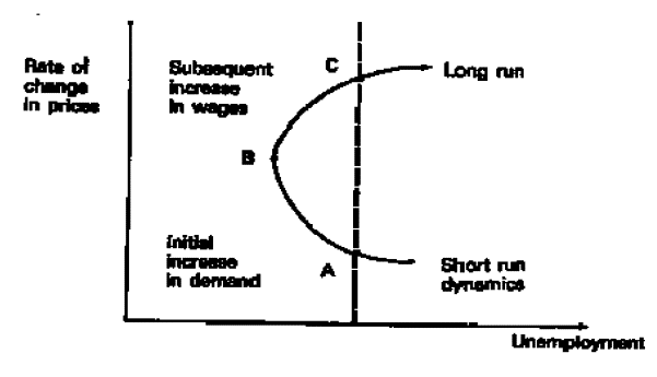 Fig5(ii): Prices and unemployment
A spurt of inflation results (figure 5) in a reduction of unemployment as the real wage is lowered. This sequence of events corresponds to the 'short-run' Phillips curve, segment AB. Subsequently, as the previous real wage is restored, unemployment increases (the economy moves from B to C) and we are left with a higher rate of inflation but the old level of unemployment. Thus, the only change that is possible in the long run is from A to C. Friedman believes that the Keynesians err in recognising only the short-run nature of the movement from A to B, and ignoring the longer run movement from B to C.
The persistence of unemployment led to the notion of the 'natural rate of unemployment' (see Fine 62 ) which is that level of joblessness that is warranted even where the market is working 'ideally' because, for example, of the need for workers to look for new jobs or because of the random and unforeseen shocks to the economic system to which adjustment needs to be made. The natural rate of unemployment (NRU) was also originally identified as that point at which inflation would not accelerate, or decelerate, along the vertical part of the Phillips curve. The persistence of unemployment and inflation in the 1980s led to the notion of the non-accelerating inflation rate of unemployment (NAIRU). This illustrates how economists moved away from Keynesian notions of full employment to concentrate upon inflation control first.
The two major causes of inflation are costs rising faster than increases in productivity and demand running higher than supply. Presumably, Friedman thinks that the latter works first and the former second. In a world that is not neo-classical, however, wage rises need not necessarily be financed through inflation but, for example, from profits and, if these were too low, from increased taxation of richer in favour of poorer workers. Workers do not necessarily demand wages in excess of productivity increases. They demand a wage which, at least does not fall in real terms. Hence, when information is poor concerning future inflation, workers will attempt to discount the future by asking for wage increases above the inflation rate plus productivity increases, thus contributing to a further bout of inflation. Certainly, the high real interest rates in the 1990s contributed to breaking this vicious circle as inflation fell, growth increased and unemployment fell. However, outside of the USA, UK and a few other countries high levels of unemployment continue to remain persistent in many industrialised countries. Solow 63 was particularly scathing of the NRU and stated "The proper conclusion is not that the vertical long-run Phillips curve version of the natural rate hypothesis is wrong. I would suggest instead that the empirical basis for the story is at best flimsy. A natural rate that hops around from one triennium to another under the influence of unspecified forces, including past unemployment rates, is not 'natural' at all. 'Epiphenomenol' would be a better adjective!'
7. Segmentation and empirical theories
A segmented labour market is one in which some workers receive higher real wages than others with the same level of human capital simply by virtue of their sector of employment. An early conceptualization of segmented labour markets came from Doeringer and Piore 64 who distinguished two main segments: a primary segment and a secondary segment. The primary segment is characterised by jobs requiring self-initiating action on the part of the worker and the secondary segment is characterised by jobs requiring the least on-the-job training, the minimum of skill and response to simple, direct orders. This conceptualization was developed for the USA but the parallel in developing countries would be modern and traditional sectors.
Segmented labour markets can result in a mismatch between workers' skills and actual requirements, and in unfulfilled demand for labour in some sectors and excess supply of labour in others. To a certain extent both the Lewis and Fei/Ranis models satisfy these conditions. However, Squire 65 criticises these models because he believes that their dualistic idea is too simple to reflect the complexity of the real world. He believes that at least three additional factors should be included, namely, first a theory of wage rate determination or a demonstration that the industrial wage (for example) is indeed determined by minimum wage legislation. Second, two sectors are not , a major development being the traditional or informal sector (see Chapter 3). Third, the assumption that labour is a homogeneous factor of production. For example, dualistic models explain unemployment and wage differentials by reference to the existence of segmented labour markets. If labour is heterogeneous, however, unemployment can be explained without reference to segmented labour markets; unemployment can exist for some types of labour (e.g. educated workers) and not for others (e.g. unskilled workers) or, more usually, vice versa. Recognition of heterogeneity makes it very difficult to interpret earning differentials. On the one hand they could reflect quality differentials, on the other they could indicate a distortion.
Segmentation between modern and informal sectors leads, in many developing countries, to rigidity whereby the transition from informal to modern by labour is rarely made. Despite the popularity of the informal sector concept as a sink sector for the unemployed and/or marginalised or, according to some commentators, one of the most dynamic parts of the economy; conceptualization of it has proved difficult. No existing formal model precisely defines the informal sector in terms of other sectors or in terms of the relations of production. Squire 66 defines the informal sector as that in which the return to labour, whether or not it be in the form of wages, is determined by the forces of supply and demand. Others define it as that sector not touched by the formal legal system of a country. Statistically, it is often defined as comprising all those who work for companies of five persons or less outside of the professions such as lawyer or architect.
Squire is not the only one who is unhappy with attempts to define the informal sector because they have been, to date, empirically based and do not fit into an overall theory. Hart, 67 for example, defines the informal sector as the province of self-employed workers and the formal sector as that of wage employment. The ILO 68 originally identified the informal sector according to a variety of characteristics, such as small-scale enterprises, or activities that rely on indigenous resources or family ownership of sector with any degree of certainty and, in consequence, makes analysis, including data collection, very untidy (see next chapter for the current definition).
Unemployment is sector specific in the Lewis model, even though the wage floor is economy wide because, in agriculture, excess workers can obtain the means to subsist. Hence, Lewis' capitalist sector workers are in open unemployment and in his subsistence sector they are in disguised unemployment or, in other words, they are underemployed (more will be said on definitions in the next chapter).
In the Harris-Todaro model 69 there is also a rigid wage but, unlike Lewis, it is not economy wide. The contribution of this model to an explanation of unemployment, is a labour allocation mechanism under which actual wages are not equalised. The actual rural wage is equated with the expected urban wage, the latter defined as the (rigid) minimum wage weighted by the rate of employment (i.e. the share of persons in this labour market who are employed). The Harris-Todaro model, then, explains why workers remain in open unemployment rather than accept a readily available job at a lower wage. Their model states that workers employed in the rural sector have no chance of obtaining a high wage job or, conversely, only those excess workers in open unemployment have a chance of obtaining a job in the rigid wage sector. Note, too, that a worker is not unemployed solely because of the absence of aggregate imbalances between labour supply and demand. Hence, in its description of the labour market, the Harris-Todaro model is neither neo-classical nor Keynesian; it can best be characterised as an empirically based theory. Like Lewis the model is, in its original form, specified so that there is full employment in the rural sector and unemployment in the urban sector. This is consistent with the fact that urban wages have continued to rise in many developing countries. With a labour supply function based on expected income, there will be open unemployment as long as a worker without a job has a higher probability of obtaining a high wage job than does a worker with a low wage job.
Educational differences in the labour market can lead to a 'cascade' model where the highly trained currently unemployed replace the less qualified, and the latter in turn replace people less qualified than them, and so on. If all unemployment were of the search rather than the queuing variety, then the unemployed would be self employed in information collection and, according to Berry and Sabot, would be optimally allocated. Now we see shades of Friedman's monetarist view in which all observed unemployment is natural for a given economy at a given time. Then the 'social' cost of a given amount of unemployment would be less than in a situation where Keynesian deficiency of demand prevails, since unemployment would be involuntary.
Educational differences in the labour market can also lead to 'mismatch'. The mismatch that has received most attention to date is the use of educated persons in positions that could be filled at lower opportunity cost by others. The problem involves the relationship between the educational and occupational levels of labour force members, and the degree to which the education system is providing workers with the appropriate skills. All this depends, of course, on the composition of the demand for labour at some future point in time.
However, more recently (Hayter and Barnes 70 ) segmentation labour market theory has suffered from two main criticisms. First, it does not have much to say about monopoly capital and second, it does not proffer an alternative theory of the competitive sector. Through occupying an 'ill-defined' theoretical terrain, at times relying on abstract explanatory variables like the industrial structure and, in consequence, it has rejected human capital theory.
8. Recent neo-classical views 71
The Washington Consensus currently dominates economic policy. For the labour market, it is argued that there are no general or plausible tractable models of imperfect competition. The tractable models always involve some set of arbitrary assumptions about tastes, technology, behaviour or all three. This means, according to Krugman, that in order to do development theory 'one must have the courage to be silly, writing down models that are implausible in the details to arrive at convincing higher-level insights'. Current theoretical work has focussed upon 'new growth theory' as created by Romer 72 and Lucas 73 . It attempted to get away from the conventional Solow result that most long-term per capita growth arises from exogenous technical progress through three related hypotheses: (1) social returns to investment are higher than private returns because of external economies, (2) capital broadly defined is a much larger share of input than conventionally measured and (3) technical progress is largely an endogenous result of market-driven research and development. Thus new growth theory has been pre-occupied with explaining the persistence of growth than how to get it started - different from high development theory that tried to provide a guide to policy.
The preoccupation with growth (and trade but not even alluded to here because the subject is so vast - I have discussed some of the aspects between trade and labour elsewhere 74 ) has assumed that employment creation is simply a consequence. This view can be attributed to Krugman who, in his review article of development economics hardly mentions employment and then only labour as a factor of production. Fine, however, draws five main conclusions on contemporary labour market theory and is consistent with the views and comments expressed in this chapter. First, it is inappropriate to examine labour markets in terms of equilibrium economics since there is no reason to presume that the forces that operate within labour markets interact more or less harmoniously and efficiently to grind out equilibrium levels of employment and associated working conditions. Second, labour markets are differentiated from one another, giving rise to empirically recognisable labour market segments or structures even though segmentation theory has tended to proceed in terms of divisions across the labour market as a whole and even though these divisions are perceived to be shifting and overlapping. Third, these labour market segments can be derived from 'horizontal' and 'vertical' factors. The former refers to determinants that prevail across all sectors of an economy, such as differentiation by gender and skill and the latter refers to the structuring within particular sectors of the economy. Fourth, with the rejection of equilibrium, it is necessary to demonstrate how labour market structures are socially reproduced, transformed or develop historically. This latter point does not mean degeneration into empiricism in which structure becomes identified mainly with large differences in behaviour as long as the structures are shown to incorporate underlying socioeconomic factors in an integral fashion. Fifth, labour market structures need to be derived from those socio-economic factors that arise out of the division between capital and labour and out of the profit imperative. This, in turn, implies a particular analytical and causal structure to labour market analysis, in which labour market structures are the reproduced and complex outcomes of the capital-output relation and its associated tendencies, such as productivity increase, deskilling, monopolisation etc.
Fine ends his discourse with the more controversial view that, within orthodox economics, the core starting point is essentially that labour is just like any other commodity i.e. it is subject to the laws of supply and demand that themselves can be derived from the marginal productivity of labour and from the marginal utility of leisure and in conjunction with optimisation over other decisions such as how much to save. However, the persistence of unemployment in market economies has influenced liberal economists to explain why wages do not immediately adjust to bring markets into equilibrium at full employment. The neo-classical paradigm is that wages will gradually adjust to bring labour supply and demand into equilibrium. In particular, the persistence of unemployment has led the neo-classicals to wonder why firms do not drop their wages, so that it becomes worthwhile for them to employ the extra workers. One reason is that unions simply prevent the firm paying less and it is noticeable that unions tend to protect those 'in' work rather than those 'out' of work - unemployment is a problem for most unions in the sense that those in work may become unemployed. A second reason is that every personnel director will tell the board that wage reduction will reduce morale and cause trained workers to quit and hence the losses from this would outweigh the savings made on lower wages. This is the 'efficiency wage' explanation.
Another way of putting this is that a firm can hire all of the labour it wants at the wage it chooses to offer so as to maximise its profits by offering the real wage which satisfies the condition that the elasticity of effort with respect to the real wage equals unity. This condition has become known as the Solow condition and the wage offered the efficiency wage since it minimises labour costs per efficiency unit 75 .
According to this view, firms may offer wages in excess of the market-clearing level to discourage labour turnover which is costly to them. The labour turnover model predicts that workers will become less likely to quit their jobs the higher is the wage paid by their employer relative to the market-clearing level and the higher is the aggregate rate of unemployment 76 .
Indeed, the persistence of unemployment after a supply shock can be partially explained by 'efficiency wage theory' 77 . Workers base their notion of a 'fair wage' upon what wages have been in the past. If an adverse supply shock reduces productivity, as after oil price shocks for instance, the 'fair' wage will not fall initially. In consequence, the profit-maximising wage will rise relative to productivity - thus, potentially, raising unemployment.
This notion of 'fair wage' has led to what is known as 'insider-outsider' models 78 . There 'insiders' in the firm can capture productivity improvements in the form of higher wages in the short run. Yet, in the face of unemployment and in the longer run, market forces re-assert themselves and wages return to their equilibrium value. One important feature of this case is that following a shift in productivity or demand, employment will change only sluggishly because of the role of insiders in wage-setting. With this sort of 'turbulence' in place of smoothly adjusting markets, there will be frictional unemployment as workers move from contracting to expanding firms.
Related to these two former models is that of the asymmetric-information models 79 . There lack of information on wages in competing markets lead to sluggishness of markets to adapt and unemployment ensues. Moreover, Grossman et.al. argue that it is the increase in uncertainty that prevents workers to change jobs, rather than information misperceptions, and this uncertainty generates the increase in equilibrium unemployment.
But, others see labour as special. Standing 80 , for instance, sees increased flexibility in the labour market having been traded for reduced security. And, Sapsford and Tzannatos 81 do see labour markets as special and theory having enjoyed considerable analytical progress over the 1980s. This progress has revolved around a focus upon the allocation of time and the notion of human capital. Finally, it does appear that the focus upon growth theory in recent years has led to questions of employment being more of an 'add-on' than a focus of economic theory per se, which differs sharply from the focus on the labour market by the classical economists and social reformers such as Keynes.
9. Concluding remarks
The main concern of this chapter has been to provide an overview of the major theories which have attempted to describe how the labour market works. This is as a precursor to the presentation of a simulation model of unemployment and to illustrate the wide divergence of opinions and theory of the determinants of labour underutilisation. The recent tendency to see labour markets as mostly clearing except for institutional factors (such as high social charges in European countries in comparison with the USA for example) is commensurate with most analysts who see labour markets as malfunctioning because of distortions in the wage rate. It is felt that if only there were an improvement in market signals, such as better information about job openings, a wage rate equal to the market clearing rate, etc., unemployment would disappear. This suggests a return to the neo-classical word of Walras, vigorously opposed by Keynesians and Marxists and characterised neatly by Freeman's presentation of the red and blue corner warriors.
III: The measurement and monitoring of mismatches (employment and unemployment)
1. Introduction
Data availability for manpower or human resource planning at the national level are poor in developing countries. Further, there is much confusion over the meaning of employment and unemployment - and this is not confined to the developing countries with frequent changes of concepts and terminology occurring in the developed countries mainly to suit the interests of one political party or another. In this chapter, therefore, the question of 'what are we trying to measure?' is examined and then the main accepted international definitions are presented and discussed. In the developing countries mismatch between what is available and what is not often leads to a large informal sector and, therefore, recent ILO work in defining the informal sector is presented and discussed.
International comparisons of unemployment give an incomplete indication of how well labour markets function from country to country. Conceptual difficulties abound and the lesser developed a country is the poorer is its labour statistical base. For instance, the OECD publishes unemployment figures as supplied to it by its member governments but these are not directly comparable across nations. Buried in the back of OECD Reports, however, is a presentation of standardized rates for comparability among members for some of its member states.
EUROSTAT has access to its member countries' labour surveys in their raw form and publishes internationally comparable statistics that uses the ILO international definition of unemployment. Table 1, for instance, shows the difference between OECD and EUROSTAT estimates for 1992. There the variations in estimates vary significantly for some countries, Belgium, Denmark and Ireland for example while the bigger and richer European countries show convergence.
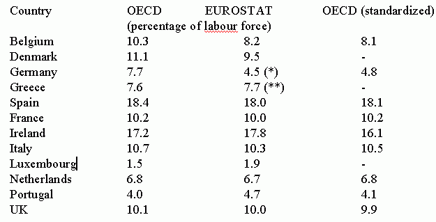 Table 1(iii): Unemployment estimates compared for 1992
Sources: OECD: Employment Outlook, July 1993
Table 1(iii): Unemployment estimates compared for 1992
Sources: OECD: Employment Outlook, July 1993
EUROSTAT: Unemployment, 5 October 1993
*The OECD figure includes former East Germany, the EUROSTAT figure not.
**read 1991 figures
Individual countries sometimes change the conceptual basis of the unemployment figures - often this is done by politicians to gain political advantage. For example, in the UK in 1982 instead of measuring the monthly total of unemployed on the basis of jobseekers registered at employment exchanges, it was decided that the total should henceforth be measured on a claimant basis. This meant that those who were not entitled to unemployment benefits were excluded from the official count. This lowered the unemployment figure by, on average, over 100,000 a month. In 1998, this was changed back to the original ILO definition as the new Labour Government came to power.
Tunisia, for example, manages to reduce its unemployment rate by several percentage points by excluding those aged 15 to 17 and 59 to 65 years of age who would normally be included in the international definition. This category is called the 'potentially employed' or 'other not occupied' and therefore excluded from the unemployment statistics. Thus, in 1980 for example, official unemployment excluded about 40,000 1517 year olds and 3,600 aged over 59 years.
A more intangible problem is the question of female employment and, in particular, the question whether women confined to the home constitute part of the active or inactive population. Again, Tunisian statisticians among others have grappled with this problem and remarked (INS, 1988) that women not only constitute an important part of the inactive population but pass easily between the active and nonactive population depending on how the survey question is phrased. For example, in the 1975 Tunisian census housewives who declared themselves inactive (and therefore not part of the labour force) were asked an additional question to determine whether they participated in remunerated activities or helped in the family business (including agriculture). In the survey of 1980 and the census of 1984 the subsidiary questions were further refined and ,thus, a substantial proportion of women who had initially declared themselves inactive were added to the labour force and the employed population. In the 1986/87 labour survey of 24,000 households the INS reversed itself and excluded housewives from the labour force. The net effect of all this is that the official unemployment figures in Tunisia are not immediately comparable from period to period.
And South Africa only includes 'formal' employment in the numerator of its unemployment statistics and these are mainly white. But it includes the black labour force in the denominator, ignoring the fact that many of these work in 'informal' type activities that, with the international definition, would be included in the persons employed figures. Consequently South Africa publishes ludicrously high 'unemployment' rates in the range 40 to 50 per cent when the real figure is probably less than 20% 82 . This does not mean that the employment problem is not severe in South Africa, simply that the problem is more one of underemployment and low labour utilization than one of unemployment per se. The implication of 45% unemployment rates has led the South Africans to worry about how to increase the number of 'formal' jobs when a more important problem is how to raise the productivity of 'informal' jobs!
2. Concepts of labour force participation and underutilisation
There is no ideal labour force concept. Standing (1981), for example, groups the concepts that exist into two main groups. One is 'basically behavioural', i.e. what people do with their time, and the other is 'basically normative', i.e. work in terms of what people actually get out of it. The labour force approach is basically behavioural, is the most widespread, and is generally recommended by the International Labour Organisation (ILO). The labour force is equal to the working age population multiplied by the economic activity rate. It is based on the distinction between active and inactive and assumes the working age population is easy to find. Each country that applies this method has a slightly different version, sometimes the working age population is defined as those over 12 years of age, or all those between 15 and 64 etc. (see Hussmanns, 1990) According to the international standards, the 'economically active population' comprises all persons of either sex who furnish the supply of labour for the production of goods and services as defined by the United Nations systems of national accounts and balances, during a specified time reference period. According to these systems, the production of goods and services includes all production and processing of primary products, whether for the market for barter or for own consumption.
The international standards, defined at regular meetings of the International Conference of Labour Statisticians (ICLS) at the ILO, use the term 'economically active population' as a generic term and identify, in particular, two measures of the economically active population: the 'usually active population' measured in relation to a long reference period such as a year; and the 'currently active population' measured in relation to a short reference period such as one week or one day - the latter term is referred to as the 'labour force'. Thus the measurement of the economically active population involves three basic conditions: the scope of the population to be covered; the dividing line between economic activities and non-economic activities; and a measurement framework for applying this dividing line to that population.
In practice the economic activity rate is based on the notion of employment which is usually defined as any occupation by which the person who pursues it receives compensation in money or in kind or in which he or she assists in the production of marketable goods and services. To be called economically active a person without work has to have been 'available and wanting work' during the specified period and also should have been actively seeking it. Clearly, this approach throws up many problems when it comes to defining an economic activity rate. First,in low income countries, and in particular in rural areas dominated by subsistence agriculture, the concept is meaningless since specialisation of activities has not developed, e.g. domestic work is excluded and so is voluntary work; sitting under a tree deciding what action to take over some local dispute would probably not called work, yet in another country similar deliberations could be the salaried employment of judges and barristers. Second, by a rigorous interpretation of the definition a beggar could be counted as gainfully employed since it is to be hoped that he or she occasionally receives compensation. So that the beggar would not be counted, gainful employment might be defined by some reference to production. But, then suppose the beggar attempts to increase his income by singing to passersby; he would be producing a service of some sorts. In that case it might seem that one could either relate gainful employment to expected demand or to the recognition aspect of employment. If the existence of demand rather than its expectation was taken as a criterion, it would tend to result in the exclusion of many lottery ticket sellers who, by perpetually pestering people, hope to stimulate a demand for their products. Third, the reference period for classifying people as working unemployed or economically inactive is also crucial. It is affected by seasonal variations, illness, holidays, absence from work, etc. Fourth, it is assumed that the aggregate labour supply can be measured by size of labour force. Yet labour supply cannot be measured simply by the number of employed and unemployed, however defined. Labour supply consists of hours, days and months; effort and intensity of work, commitment to specific jobs and continuity of work. Measurement can be improved by measuring hours worked. However that ignores those who work long hours for meager rewards, e.g. newspaper vendors, shoe shiners etc.
The following approaches have been suggested as a response to the above criticisms of the labour force approach and, following Standing, can be termed normative.
2.1. Subemployment index
The open unemployment rate is an inadequate index of labour underutilisation because it treats all employed and unemployed as supplying an equivalent amount of labour. Many people measured as employed may be working at a lower level of production, or working for shorter periods and less intensively, than they would be able and willing to work. Because of this the Gordon report (United States, 1962) suggested using a 'subemployment' index. This was to include the unemployed, discouraged workers, people working part-time who wanted full-time work and family heads who did not earn enough to keep their families out of work. Myrdal(1968) suggested discarding entirely the concepts of 'unemployment' and underemployment' as inadequate to reality. Concepts should be based on simple behavioural notions: which people work at all, for what periods during the day, week, month,year, with what intensity and effectiveness, etc.
2.2 Basic needs approach
Elsewhere, the author has suggested that un- and underemployment exist in all families who do not satisfy their basic needs (Hopkins, 1980). Hence, even individuals who appear, according to conventional definitions, to be openly unemployed (e.g. educated workers waiting for jobs, frictional employment, etc.), but belong to families whose basic needs have been satisfied are excluded from the ranks of the un- and underemployed with this definition. A major problem, of course, is what to define as basic needs, what indicators to use and at what level they should be set. This I have discussed also elsewhere (Hopkins, 1983). Given that basic needs can be defined - I have defined them in terms of adequate nutrition, housing, education and health - the method has an advantage in terms of its analytical tractability. This is because a household income that would enable purchase of the physical goods in the basic needs basket can be calculated. Given reliable consumption expenditure information, an estimate of un- and underemployment can be constructed. Policies can then be examined as to how they could satisfy basic needs. Such an approach means concentration on the genuinely underprivileged rather than, perhaps, generating employment in areas where, according to my definition, it is not needed. This brings us into the controversy of whether increasing productive employment opportunities is equivalent to satisfying basic needs. If, under conventional definitions, those who are un- or underemployed have not satisfied their basic needs then the set of policies would be equivalent. If, however, those who are not considered un- or underemployed have also not satisfied their basic needs and if those who are un- or underemployed have satisfied their basic needs , then the two sets of policies are not equivalent. Often poverty and unemployment go hand in hand (for India see Pravin Visaria, 1981).
2.3 Labour efficiency approach
Myrdal (op.cit.) proposed that the level of labour utilisation be expressed as the product of three ratios, viz.

Underutilisation of the labour force is the non-achievement of those values of the three components of labour utilisation which can reasonably be assumed to be brought about by feasible policy measures during a planning period. Clearly, the measurement here introduces as many problems as the labour force approach because it is impossible to define what is reasonable and feasible.
2.4 Symptomatic approach
The attempt here is to measure labour underutilisation based on a classification of different types of underemployment. The one recommended by the ILO is:
-
Visible underemployment - involuntarily working part-time or for shorter than usual periods;
-
invisible underemployment - working time is not abnormally reduced but unemployment is inadequate because:
-
the job does not permit full use of a person's highest skills or capacities;
-
earnings from employment are abnormally low;
-
employed in an establishment or economic unit whose productivity is abnormally low.
(i), (ii), (iii) are disguised underemployment. However, a more rigorous definition of disguised underemployment might lead to the conclusion that most workers in most countries of the world are invisibly underemployed because the definitions are phrased in vague terms such as 'abnormally', 'usual periods of work', etc.
2.5 The Hauser approach
This method (Hauser, 1972) is a variant of the symptomatic approach. Hauser suggests that the workforce be divided into two parts: utilised adequately or underutilised. The latter is to be further subdivided into four parts: underutilised by employment, by input, by productivity, by mismatch of occupation and education. All people with less than full-time work are to be classified as underutilised. Further, all those reporting full-time work whose income falls below an income level determined to be a suitable point for policy and programme purposes, are to be classified as underutilised by productivity. Problems arise here because not all those working short weeks want to be, or are capable of, working full-time or full weeks. Second, in terms of mismatch, there is difficulty in defining compatibility. Hauser suggested the mean educational level for each occupation should be the yardstick, but there is no reason to suppose that this would reflect the appropriate amount of education for a specific occupation (e.g. on-the-job skill acquisition). Moreover, it is a mismatch if a worker has an education compatible with his/her occupation but is nevertheless unable to work as much as he/she might want, or is earning less than he/she might reasonably be expected to earn in that occupation.
3. Employment definitions currently applied
The labour force framework supported by the ILO and the one generally accepted worldwide, gives rise to three main categories - unemployment, employment and economic inactivity. The former two are looked at, next, in turn. Since the three concepts are mutually exclusive, all those who are neither employed in some sense nor unemployed are said to be economically inactive and this is therefore the residual category.
3.1 Unemployment
The conventional definition, and the one most widely used today, was agreed upon by labour statisticians in the 1982 ILO conference on the subject. Briefly, it sets three separate criteria for classification as unemployed. The unemployed must be first be without work, second currently available for work during the reference period; and third seeking work, that is, must have taken specific steps in quest of a job during a specified recent period.
Thus, the unemployed comprise all persons above the age specified for measuring the economically active population who during the reference period were:
-
'without work', i.e. were not in paid employment or self-employment, as specified by the international definition for employment;
-
'currently available for work', i.e. were available for paid employment or self-employment during the reference period;and
-
'seeking work', i.e. had taken specific steps in a specified recent period to seek paid employment or self-employment.
Special provisions are made for persons without work who have made arrangements to start work at a date subsequent to the reference period and for persons whose employment contract is temporarily suspended.
The without work criterion draws attention between employment and non-employment. 'Without work' should be interpreted as total lack of work, or, more precisely, as not having been employed during the reference period. The purpose of the without work criteria is to ensure that employment and unemployment are mutually exclusive. A person is classifiable as unemployed only if it has already been established that he or she is not employed. Thus persons who were engaged in some casual work while seeking employment should be classified as employed, in spite of the job search activity. The other two criteria of the standard definition of unemployment, 'current availability for work' and 'seeking work', serve to distinguish those of the non-employed population who are unemployed from those who are not economically active.
There are many difficulties and subtleties in the application of these seemingly simple rules. Perhaps the most contentious is what is meant by 'without work'. Internationally this is accepted to be a person in the reference period, which is usually one week or one day before the survey question is posed, who did not work for pay or in-kind earning for even one hour.
Recognizing that too exclusive a focus on a single measure may distort the view of other developed nations in comparison with that of the United States, the US BLS (Bureau of Labour Statistics) has published since 1976 seven alternative measures for unemployment. Briefly, the data go from a very restrictive definition of unemployment (U-1), past the ILO standard definition (U-5) to a definition of unemployment that is very broad and includes discouraged workers for example (U-7). Sorrentino (1993) applied these definitions to nine countries and found that the unemployment rate varied for the US from 1.2% to 7.9% (U-1 to U-7), 8.1% to 11.1% for France, 1.5 to 9.3% for the UK and 0.4 to 7.2% for Japan for example. These striking results led Sorrentino to conclude for 1989 that there are, unsurprisingly, major labour market differences among North America, Europe, and Japan but, more surprisingly, Sweden and Japan have the largest increases in unemployment when part-time work for economic reasons and discouragement with the labour market are taken into account. In these two countries, labour slack moved much more into involuntary part time employment and discouragement with the labour market than into open unemployment. Joblessness of long duration was found to be much more prevalent in Europe than in North America, but North America was seen to have more job losers, reflecting the lower level of job security in the US and Canada, compared with Europe and Japan.
3.2 Employment
According to the ILO's 1982 international definition of employment agreed at the Thirteenth International Conference of Labour Statisticians 83 (Thirteenth ICLS), the 'employed' comprise all persons above the age specified for measuring the economically active population, who during a specified brief period (one week or one day) were in the categories:
-
paid employment (1) 'at work' persons who, during the reference period, performed some work for wage or salary, in cash of in kind; (2) 'with a job but not at work': persons who, having already worked in their present job, were temporarily not at work during the reference period but had a formal attachment to their job;
-
self-employment (1) 'at work': persons who, during the reference period, performed some work for profit or family gain, in cash or in kind; (2) 'with an enterprise but not at work': persons with an enterprise, which may be a business enterprise, a farm or a service undertaking, who were temporarily not at work during the reference period for some specific reason.
The international standards further specify that, for operational purposes, the notion of 'some work' may be interpreted as work for at least one hour! The one hour criterion, although not explicitly recommended is implicit and is to cover all types of employment that may exist in a given country, including short-time work, casual labour, stand-by work and other types of irregular employment. It is also a necessary criterion if total employment is to correspond to aggregate production. In employment projections, labour force planning and productivity calculations one usually needs to link measured production in a given industry to the total labour input for that production. Since all types or production falling within the production boundary are in principle included in their totality in national accounts, it follows that all corresponding labour input, however little it may be in terms of hours worked, should also be accounted for. An increase in the minimum number of hours worked in the definition of employment (and thereby unemployment) would distort such analyses.
3.3 Further disaggregation
One reads in the economic literature of additional disaggregations of unemployment. Urrutia (1968), for example, suggested that unemployment should be further disaggregated into frictional unemployment and structural unemployment. The former occurs in an economy with high labour mobility, e.g. through population growth, migration and new entrants; there is likely to be a certain amount of unemployment as these people look for work. Such unemployment is of short duration and could be reduced, according to Urrutia, through improving the generally poor information on employment opportunities. Frictional unemployment is thus relatively unimportant compared with structural unemployment. The latter covers people in regions with a dim economic future, those with skills not necessary for the system of production, old people,the sick, the infirm, those suffering from poor nutrition, etc. The social cost of this form of unemployment is very high because it is more or less permanent, or at least of long duration. It can be avoided, according to Urrutia, through a number of measures such as regional employment subsidies, public works, re-education schemes, programmes of employment for senior citizens, and subsidies to firms who employ such workers.
To these two categories, Marshall (1976) would add cyclical unemployment. This occurs because of the general slackening of demand during recessionary periods and also includes seasonal variations in demand. Usually, the burdens of cyclical unemployment are spread widely, and even employed workers are likely to suffer from reduced weekly hours and/or reduced take-home pay.
Two further concepts have been widely used during recent times, viz. additional and discouraged workers. When there is a fall in demand for labour, implying a lower return per unit of time spent in the labour force, the result is an additional worker effect in that families affected attempt to make up for what they consider to be a transitory decline in income, by increasing the number of household members (mainly married women) in the labour force. If the size of the labour force declines as the level of unemployment rises, those workers who leave the labour force are known as discouraged workers and are in the state of disguised unemployment. Standing (op.cit.) names six types: (i) discouraged jobseekers; (ii) those inhibited from entering or re-entering the labour force; (iii) those who adjust the timing of their partial labour force participation; (iv) laid-off secondary workers whose attachments to the labour force is very weak, even when unemployment is cyclically low; (v) those who retire earlier than anticipated; and (vi) those who remain in, or reenter, education as a response to unemployment.
3.4 Underemployment
According to the 1966 ICLS resolution, underemployment exists 'when a person's employment is inadequate, in relation to specified norms of alternative employment, account being taken of his occupational skill (training and work experience)'. Two principal forms of underemployment are distinguished: visible underemployment, reflecting an insufficiency in the volume of employment; and invisible underemployment, characterised by low income, underutilisation of skill, low productivity and other factors. The 1982 ICLS resolution weakened the emphasis on underemployment by noting that 'for operational reasons the statistical measurement of underemployment may be limited to visible underemployment'.
The international definition of visible underemployment comprises 'all persons in paid or self-employment, whether at work or not at work, involuntarily working less than the normal duration of work determined for the activity, who were seeking or available for additional work during the reference period'. This means that visible underemployment is defined as a subcategory of employment and that there are three criteria for identifying, among persons in employment, those who are invisibly employed: (1) working less than normal duration; (2) doing so on an involuntary basis; and (3) seeking or being available for additional work during the reference period.
The 1982 ICLS noted that compared to invisible underemployment, which is a statistical concept directly measurable by labour force and other surveys, invisible underemployment is 'primarily an analytical concept reflecting misallocation of labour resources or a fundamental imbalance as between labour and other factors of production'. To measure invisible underemployment, whether in respect of income, levels of skill or productivity, it is necessary to establish thresholds below which the income is considered abnormally low, the skill underutilised, or the productivity insufficient. Despite these problems, some countries have attempted to measure various aspects of invisible underemployment by using the framework developed by Hauser (see above) by using his labour underutilisation framework. It has been applied mainly in South-East Asian countries (Hong Kong, Indonesia, Malaysia, the Philippines, Singapore and Thailand). As Hussmanns et.al. note, it has been an attempt to measure the inadequacy of employment in a broad sense, covering not only invisible underemployment in terms of level of income and use of skill, but also visible underemployment and unemployment. However, the concept has not so far been endorsed by the ICLS because of the difficulty in defining international standards. At the fifteenth ICLS in 1993, the ILO noted that the experience of many countries on the measurement of underemployed in terms of time worked (visible underemployment) were of limited relevance in describing the employment situation. For instance, in situations where many persons receive low incomes although they are fully employed in terms of time worked, or in situations where a large proportion of the labour force is self-employed and where a lack of demand for their products tends to result in low intensity of work and low income rather than a reduction in the time spent. The ILO proposed to continue investigating this subject and to present its findings at a future ICLS.
3.5 Informal sector employment
The concept of the informal sector has played a growing role over the past three decades, in particular, in developing countries for its alleged role in absorbing vast numbers of unskilled labour in a dualistic economy. It is surprising, therefore, to note that no clear and generally accepted definition of the concept exists. Recently, the ILO ICLS has begun to take the concept seriously and preliminary deliberations have taken place under the form of the Meeting of Experts on labour Statistics (MELS). They note that one may broadly characterise it as the aggregate of activities that result from the need for generating one's own employment to earn a living because other sectors of the economy - agriculture, large modern firms and the public service - are unable to provide a sufficient number of adequate employment and income opportunities for a rapidly growing labour force and there are no - or only rudimentary - social benefits from the State to fall back on. It is by no means a marginal phenomenon - rough estimates put it at 300 million in developing countries (ILO, 1991) . In developed countries, the labour surplus is smaller and social protection systems exist and therefore the informal sector that does exist (eg small-scale units outside the formal economy or services rendered by one household to another) is small. Additionally, many activities exist in the black or concealed economy. In Central and Eastern Europe and some of the Southern European countries, the black economy is widespread.
The informal sector in developing countries typically consists of very small-scale units established and owned by self-employed persons either alone or in partnership with others. They often have very little capital, equipment, technical know-how or managerial skills, and use simple, labour-intensive technology (Tokman, 1991). As a result, most of these units work at low levels of organisation, productivity and income. They tend to have little or no access to organised markets, credit institutions, formal education and training, or public services and amenities. The vast majority of these activities are legal in themselves, i.e. they provide goods and services whose production and distribution is perfectly legal such as handicrafts, vehicle repair, taxi driving, food selling etc. this is to be contrasted with criminal activities or illegal production e.g theft, extortion, smuggling, production and distribution of drugs, prostitution etc.
On the other hand, governments often tolerate the existence of informal sectors performed outside or at the fringe of laws and regulations because they lack the means to cover the whole economy with legislation or because they realise that many informal sector activities will one day become legal. Indeed, among informal sector entrepreneurs there is a desire to legalise their operations whenever possible, since this would enable them to have access to some institutional support, such as credit, or to the protection of the law in such matters as enforcement of contracts.
The MELS have proposed a cumbersome, albeit tentative, definition of employment in the informal sector. In summary, it is as follows:
-
The population employed in the informal sector comprises all persons who, during a specified reference period, were employed in an economic unit belonging to the informal sector.
-
The informal sector consists of a group of economic units which, according to the definitions provided in the United Nations System of national Accounts (SNA), form part of the household sector as unincorporated enterprises (i.e. non-registered as a corporation or non-registered for fiscal or national accounting purposes).
-
For purposes of data collection, the informal sector comprises all household enterprises irrespective of size or type of premises used.
-
The definition can be extended to include micro-enterprises which are private, unincorporated and employ one or more regular employees while operating on a scale below a certain level e.g. such as number of regular employees.
-
The scope of the informal sector should be restricted to economic units which produce goods or services for exchange or sale on the market and which are only or mainly engaged in activities other than agriculture, hunting, forestry and fishing. Economic units owned or operated by self-employed professionals or technicians should normally be excluded.
The 1993 ICLS adopted most of these recommendations in a draft resolution produced in its January meeting. The associated documents are cumbersome and as the draft definition illustrates leaves much to individual surveys or governments to decide on criteria. The ILO was urged to carry out a number of surveys to give meaning to the definition and revisions would obviously flow. This work continues although the 1993 recommendations have now been adopted (Charmes, 1998).
4. Occupation and skill
One of the most difficult areas in manpower planning is the allocation of jobs into an occupational classification. Occupation, according to the ILO (Hussmans, 1992), refers to the kind of work done during the reference period by the person employed (or the kind of work done previously if unemployed), irrespective of the industry or status in employment of the person. Information on occupation provides a description of a person's job which, in turn, is defined as a set of tasks and duties which are carried out by, or can be assigned to , one person. Clearly the precise dimensions of a job are required when examining unemployment, wages and their evolution over time. However, the characteristics and type of job change over time as technology makes some jobs obsolete, refines others and creates new ones. In most developing countries the occupations listed are normally too aggregated to provide a detailed list of unemployed by occupation that would allow training courses to be identified as a result of a manpower planning exercise. In Vietnam, for instance, only 32 occupations are listed in their annual labour survey covering such occupations as enterprise director, culture/art officer, mining/coal/oil technology related, machine-manufacturing/electric and electronic, etc. While the number of occupations probably number in the tens of thousands.
Some clues about the occupations likely to be in demand can be obtained by looking at data on those with technical secondary education and zero unemployment levels. This actually occurred in Vietnam (see Chapter VI for full details of the exercise carried out) in eight occupational classifications - enterprise director, metallurgy/mould/coke refining, paper industry related, building material production, printing, leather/artificial leather based, aquatic breeding and harvesting, lifting machine controlling. These categories also have zero unemployment for those with a university or college education. Thus the sorts of occupations that, in 1997, had zero levels of unemployment were those with high skill or education levels such as small or medium enterprise director, graphic design linked with printing, aquaculture, high quality leather products, high quality paper products. However, a weakness in this particular methodology is that the economy might not support these occupations in large numbers - leather for instance is rare in Vietnam, aquaculture requires an unpolluted environment etc. Thus, before recommending these occupations too fervently it would be useful to look at other labor market signals such as wage levels, growth in employment, technological change in these occupational categories. For this would require more detailed occupational data plus the associated socio-economic labor market signals.
What sorts of occupational classification to use has been addressed by the ILO (Hussmans, 1992). They see an occupational classification rather like a system of maps for a country - the top level of the hierarchy being such groups as legislators or professionals going down to a lowest level where specific occupations are named such as criminal trial lawyer or pediatric doctor. Each country will have slightly different sets of occupations but it is generally seen as an advantage to have one standard national classification or occupations to be used a reference. Consequently, a standard national occupational classification is usually designed to serve several purposes. The most recent international classification is ISCO-88 (International Standard Classification of Occupations) which updates the previous one done in 1968, ISCO-68. Briefly, ISCO-88 groups occupation into four levels of aggregation - 10 major groups subdivided into sub-major groups, minor groups and unit groups. Occupations are grouped together mainly on the basis of the similarity of skills required to fulfil the tasks and duties of the jobs. Two dimensions of this rather difficult to define concept are used: skill level, which is a function of the range and complexity of the tasks involved and skill specialisation, which reflects type of knowledge applied, tools and equipment used, materials worked on, or with, and the nature of the goods and services produced. Nevertheless, despite the attention to detail in the classification system, the largest source of error in occupational statistics lies in shortcomings of the verbatim raw material as elicited and recorded in the field (Hussmans, 1992). Another source of controversy, carried out within the ILO itself (see Standing, 1999), is about the notion of labour, work and jobs. People wish to work in jobs but do not wish to labour. However, the occupational classifications struggle to define occupation and have not yet started with the task of determining which jobs are work and which are labour.
5. Concluding remarks
The manpower planner is often confronted with data which purport to measure underlying concepts but often have only a nod in the direction of precision. This chapter has covered in broad terms some of the key definitions and some of their lacunae. Not only are the methods that the manpower planner has to use severely criticised s(he) is also forced to walk on marshy ground as far as data are concerned. Nevertheless, the need for information about the future evolution of the labour force and occupations is there which is why, in the next chapter, despite the poor quality of data and conceptualisation in the labour sphere it is thought that the modelling of the manpower problem is a useful activity. It not only reveals alternative, albeit speculative, scenarios of the future it also reveals the underlying weakness of the data since a model forces data to be consistent and thereby reveals its main weaknesses.
References
- Jacques Charmes: "Informal Sector, Poverty and Gender: A Review of Empirical Evidence", Background Paper for the World Development Report 2001 (World Bank, Washington DC, Oct. 1998)
- P. Hauser: 'The work force in developing areas', in I. Berg (ed.): Human resources and economic welfare (New York, Columbia University Press, 1972),pp. 142-161
- M. Hopkins: 'A Global Forecast of Employment', in International Labour Review (Geneva, ILO), Sep-Oct. 1980.
- M. Hopkins and R. Van Der Hoeven: Basic Needs in Development Planning (London, Gower, 1983).
- R. Hussmanns, F, Mehran, V. Verma: Survey of economically active population, employment, unemployment and underemployment, (ILO, Geneva, 1992).
- ILO: The dilemma of the informal sector, Report of the Director General (Part I), International Labour Conference, 78th Session 1991, Geneva.
- INS: Enquete Nationale Sur L'Emploi en Tunisie, 198687, May, 1988.
- Marshall, Cartter and King: Labour Economics (Chicago, Illinois, Richard D. Irwin, 1976).
- G. Myrdal: Asian Drama (Harmondsworth, Middlesex, Penguin Books, 1968), Vol.2
- C. Sorrentino: 'International comparisons of unemployment indicators', Monthly Labor Review, (Vol. 116, No.3, March, 1993)
- Guy Standing: Labour Force Participation and Development, (ILO, Geneva, 2nd ed., 1981)
Tokman, V.E., 1991 'The informal sector in Latin America: From underground to legality' in: Standing, G. and Tokman, V.E. (eds.): Towards social adjustment: Labour Market issues in structural adjustment (Geneva, ILO).United States: Measuring employment and unemployment: The President's committee to appraise employment and unemployment, (Washington DC, 1962)
- Guy Standing: Global Labour Flexibility: Seeking Distributive Justice, (Macmillan, Basingtoke, UK, 1999)
- M. Urrutia: 'Métodos para medir los diferentes tipos de subempleo, y desempleo en Colombia', in Empleo y Desempleo en Colombia (Bogota, CEDE, Ediciones Universidad de los Andes, 1968).
- Pravin Visaria: 'Poverty and unemployment in India: An analysis of recent evidence', World Development (Oxford), 1981, No.3.
V: An application of the MACBETH model to labour market and human resource analysis in Sri Lanka
1. Introduction
The objective of the calibration of the MACBETH model in Sri Lanka, described in this chapter, was to assess the implications of alternative growth paths on employment and (broad) skill requirements 89 . The chapter is organised as follows. The next section presents the basic data used to calibrate the model, the second section describes the reference or base scenario to the year 2000. Then, five alternative scenarios are presented in section four and the chapter ends with a summary and conclusion.
2. Calibration of the model
In the Sri Lanka application, the model was disaggregated into 5-year age groups of population and sex. The other main disaggregations were:
-
occupations (8): professionals, administrators, clerical staff, sales workers, service workers, agricultural workers, production workers and other services including those not classified elsewhere.
-
economic sectors (8): agriculture, manufacturing, construction, utilities, trade, banking, public administration, other services and non-identified activities
-
education levels (4): no education and incomplete primary, incomplete secondary, GCE 'O' or completed secondary, 'A' level holders and University graduates.
Readers familiar with both Sri Lanka and labour market analysis might ask why there has not been a disaggregation into at least urban, agricultural and estate sectors. They might also question why informal sector activities are not identified and why private and public enterprises are not distinguished given the privatisation aims of the Government. This was because data were not available that provided consistent accounts for labour force, employment, production or value added and investment series for these issues. Thus the economic sectors and occupational classifications retained come directly from how the census has decided to classify sectors and categories. The results and conclusions of this chapter draw attention to some of the areas where data and analysis could be improved.
A full description of the equations and structure of the MACBETH model was given in the previous chapter. In Sri Lanka to obtain labour supply, a population model projects population by sex and age using the component projection method. The change in population arises from functions for fertility, mortality and external migration. The population is tracked as those of age five, or thereabouts 90 , enter into school for the first time. Students can attend five years of primary school, then enter six years of secondary school at which point they take the 'O' level examinations. Those who succeed then pass into two years of further secondary school to take the 'A' level exam and then those who pass continue into three years of higher and university education. The possibility of working and then entering or receiving skill training is not modeled. At each level of education students can repeat a grade, graduate, dropout or die.
The active population is defined to be those aged 10 to 65 and, as we have seen, the model uses a concept called 'labour pool' which is those people who are in the work ages 10 to 65 and not in school. This is disaggregated into four education levels, incomplete primary education, incomplete secondary, completed secondary and with 'O' level pass and higher education including those with 'A' levels, dropouts from higher education as well as university graduates.
Labour force participation rates are then applied to the eligible age group in the labour pool to obtain the labour force by education level. Labour force participation rates can vary over time to reflect trends such as increasing female participation for the higher educated. A matrix of education by occupation coefficients is applied to obtain labour supply by education and occupation levels.
On the demand side, employment is determined as a function of economic growth. This is done as follows. The proportion of GDP in one year dedicated to investment is calculated and then distributed among economic sectors. Incremental capital output coefficients distribute this investment into next years value added. Over time the efficiency of new investment into value added can be varied according to a user defined elasticity. Labour demand is determined by dividing value added by labour output coefficients. These coefficients change over time following past trends in labour productivity growth. This process gives employment by sector.
Employment is then disaggregated into labour demand by education by sectoral education employment coefficients. These coefficients are allowed to change over time by exogenously entered growth rates to reflect both the inflation in educational requirements over time as one way of screening job applicants and to reflect the need for higher levels of education because of technical progress. Thus the demand for employment is very flexible in order to take account of the complexity of the labour market. However, the labour function is designed to use exogenous coefficients and this was what was done in Sri Lanka. A better approach (not done) would be to estimate these coefficients exogenously to the model based on a simple regression model or an analysis of trends.
The demand for labour by occupational level is determined by a sector occupation matrix of labour demand coefficients. In alternative scenarios it is advisable to change these coefficients over time. Past trends are not always an accurate guide to how these coefficients will change since technical progress is difficult to anticipate - countries such as Sri Lanka can leapfrog through the use of acquired technology from abroad - and there is little doubt that occupation and educational requirements are likely to change at a faster pace in the future than the past. In the case of Sri Lanka the choice of occupational categories used in the census are of limited usefulness for occupational analysis - for example, the category agricultural workers does not tell us much about the composition of different types of skilled workers needed in agri-businesses, an area of activity that the Government would like to encourage. It is possible to disaggregate the model further to focus on specific occupations such as highly qualified personnel and then to lump less essential or easily substitutable occupations in one category. In the absence of such disaggregated data in Sri Lanka these issues could not be explored.
Unemployment by educational level or occupation is calculated as a residual between labour demand and labour supply. Unemployment or surplus labour is denoted by positive quantities while labour shortages are denoted by negative quantities. Surpluses or shortages of labour by education and occupation levels provide signals for the labour mobility sub-module of the model. In practice because of the aggregate way in which occupational levels were defined in the Sri Lankan census, and consequently the model, neither occupational nor educational mobility could take place.
The base year for model simulations was chosen to be 1986 since this was the latest year, at the time of the project, for which employment data was available from the labour force survey 91 (henceforth SEL). Data are discussed here for the base year as well as the parameters that give the base scenario dynamics. Full input parameters and detailed results are not given since this would make the chapter too long, however summaries are given.
3. Base year data for MACBETH
3.1 Population
No accurate data for population by age and sex were available from the 1981 census. The population projection model of MACBETH was used to project this data forward in time to 1986. The initial population data retained is given in Table 1, and the base projection to the year 2000 in Table 2.
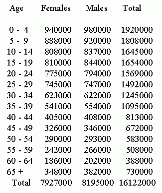 Table 1(v): Initial population by 5year groups for 1986
Exogenous Parameters for Projection of Population

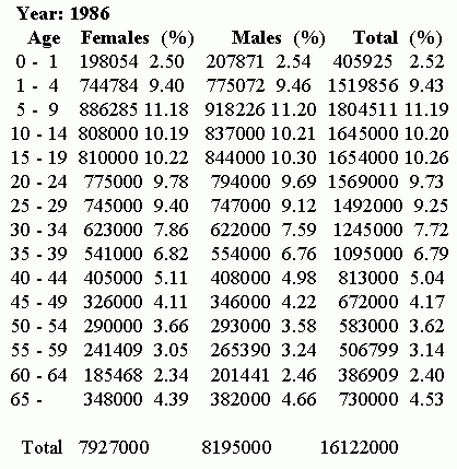
 Table 2(v): MACBETH - Projection of population for Sri Lanka
Source: MACBETH model projections
Table 2(v): MACBETH - Projection of population for Sri Lanka
Source: MACBETH model projections
Originally the population model was calibrated using data from the publication Population Statistics of Sri Lanka (PS) published by the population division of the Ministry of Health and Women's affairs in 1990. However, more recent information, at that time, from the Census and Central Bank departments, based on the 1986 contraceptive prevalence survey, showed population growth to be lower than had been originally assumed. Rather than re-calibrate the model (the impact of small changes in population growth, as will be seen, is small on labour force and unemployment), the total fertility rate data of the Census and Central Bank for 1986 of 2.6 was used rather than the original estimate of 2.8 from PS. Following the census the total fertility rate was chosen to be 2.1 in 1996.
Outward international migration data for 1986 came from the Statistical Abstract 1989, published by the Census and Statistics Department which, in turn, came from the Registrar General's office for vital population statistics. The figure 0.22% of total population migrating abroad for 1986 was based on informed judgement and noting that the figure over the period 1986-1990 varied between 0.1 and 0.3%. Life expectancy at birth for females was 72.2 in 1986 and 68.3 for males. The PS life expectancy estimates of 69.2 for males and 73.1 for females for 1996 were used. The impact of outward female international migration has led to less females than males in the population despite the higher life expectancy of females compared with males.
Given that the population model used here was not prepared with the same accuracy normally associated with population projection models (for example Model West mortality tables were used instead of tables especially prepared for Sri Lanka) the projections compare well to more sophisticated (and consequently more time consuming) projections. The estimate used here of total population for 1986 was 16.122mn compared with the census 16.117mn and 16.861mn in 1989 compared with the census department's projection of 16.806mn. By the year 2000 the estimate of total population was 18.942mn and growing 1% a year or 0.76% a year if international outward migration is included. The PS publication gave a population of 19.058 for the year 2000 but this was superseded by the census department since it was considered too high. New projections for the year 2000 were not published, at the time, but the figure used here for the year 2000 thus seems to be in the same ball park as more recent thinking on population change with a population growth rate of the order of 1 percent a year in the year 2000.
3.2 Education
Ninety percent of children enter the education system at the age of five (90%). The model also allows children to enter the first grade at the ages of six (7%), seven (2%) and eight (1%) - the percentages in brackets give the percent spread of ages as children enter the first grade. No data are available for this spread and 'judgement' was used to obtain the data. Sixteen grades of education were considered and dropouts and leavers who neither die nor migrate but were at least ten years old went into four 'labour pools' - incomplete primary, incomplete secondary, completed secondary with 'O' level pass and higher education which includes 'A' level passes, university dropouts as well as university graduates. The term labour pool is not generally found in the international literature but is used here to denote those of working age not at school.
A problem that took considerable time to resolve was the match between the education system and the labour market (this is a problem common to databases in developing countries). The solution adopted for the base run is not entirely satisfactory as can be seen from the educational data displayed in Table 2A. The initial education data from the Ministry of Education (MoE) had to be significantly 'adjusted' in order to provide sensible results (tested by matching the 1987 forecast from the model with actual 1987 data). As the first part of Table 2A shows, reasonably good agreement is achieved for the base run in 1987 and the MoE figures for the same year, with most of the estimates within one percent of 'actual' values. However, in order to ensure that the labour force by education level grew at rates agreeing with historical tendencies and were 'sensible' a number of the rates, as demonstrated in Table 2A, were changed 92 . By 1996 this led, as shown in the lower part of Table 2A, to a reasonable projection for the first 11 grades with an error that ranged from -5 to +5% in 1996, and large inconsistencies for the 12 and 13th grades. Projections were not available to assess grades 14-16. As can be seen from Table 2A, compared with the original rates, the dropout rates were lowered, and graduation rates for 'O' level passes and repetition rates raised compared with the original data obtained from the Ministry of Education. All these changes reinforced the discrepancies between the projections for the 12th and 13th grades but led to more accurate behaviour of the labour supply by education category.
The main problem that arose was that the structure of the education data originally retained led to a rapid increase in incomplete primary labour supply. Originally it was thought that this was because the repetition rates were too high and the dropout rates too low. The model was re-run several times with raised repetition rates and lower dropout rates. But these changes were not sufficient and it was eventually discovered that there was too high a retirement rate of skilled workers instead of unskilled ones and the rates were changed accordingly. This shows that, in the absence of reliable data, much experimentation must take place to get a consistent set of input parameters and a sensible base run. The inescapable conclusion is that the education statistics were incompatible with the labour force statistics. In Sri Lanka it is therefore clear that consistency checks of flows of educated people by age and grade out of the education system are not matched with flows into the labour pool and labour force.
 Table 2A(v): Education Projections
Source: Class 113 School Census 1986,1987.
Table 2A(v): Education Projections
Source: Class 113 School Census 1986,1987.
Class 1416 Statistical Handbook 1986, Statistics on Higher Education in Sri Lanka,
University Grants Committee
Class 1820 'Judgement' estimate.
* Data Not Available
Revised Base Scenario - Input Parameters

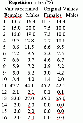

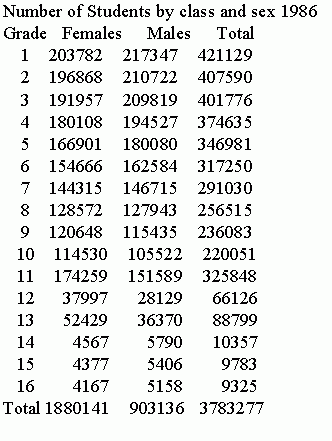 Base Scenario enrolment projections for 1986 & 1987
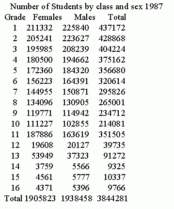
 Comparison of MACBETH & Education Dept. projections
Source: MACBETH model projections
Comparison of MACBETH & Education Dept. projections
Source: MACBETH model projections
Educational recurrent and capital cost data are used in the model and this came from the Ministry of Education. However, the focus of the work of the Human Resource group in The Ministry of Planning was labour and not educational costs, and thus no effort was made to see whether the input data corresponded with actual fiscal data for education. The data were included simply to demonstrate that the model can assess educational budgets.
3.3 Employment
Data to calibrate the labour market system came from the 1985/86 Socio-Economic Labour Force Survey conducted by the Census and Statistics Department. For a review and discussion of the labour concepts underlying this survey and how it compares with previous years see P. Alailima (1991) 93 . Following the 1985/86 survey the working age range for the labour force was chosen to be 10 to 65 (inclusive). In 1986 this survey gave an unemployment rate of 14.0% from a labour pool of 6.016mn, a labour force of 6.016mn and employment of 5.175mn. Unemployment by each of the labour categories selected were 6.7, 15.1, 22.9 and 27.4 percent going from the lowest educated to the highest respectively. Similarly, the percentage of the labour pool in the labour force for each educational category were 50.4, 58.8, 64.7 and 85.6 percent. Employment data for other variables taken from the 1985/86 survey are given in Table 3.
Distribution of employment among sectors (%)
 Table 3(v): Initial Employment Data
Distribution of education levels within sectors (%)


Variables that did not come from the 1985/86 labour in Table 3 were annual rates of change of labour requirements, labour force participation in ten years, labour productivity, wage data and years of training. The first and last of the variables in the list came from personal judgements. The labour force participation rates were based on the 1985/86 labour survey but parameterised so as to give the initial labour force for 1986. Table 4 reproduces a table from Alailima that shows changes in participation rates by educational level from three labour surveys over 1971, 1980.81 and 1985/86.
 Table 4(v): Labour Force Participation Rates by Education and Sex
Source: Dept. of Census & Statistics (1976), (1982) and (1990).
Table 4(v): Labour Force Participation Rates by Education and Sex
Source: Dept. of Census & Statistics (1976), (1982) and (1990).
No clear pattern emerged to help us decide where participation rates were heading. Participation rates were higher for the higher educated as might be expected and higher for males than for females. The trend was not clear since female participation rates rose sharply over 1980/81 to the mid 1980s but dropped for some educational levels for females between 1971 and 1980/81. The same pattern was also observed for males. The assumption retained for forecasted labour force participation rates in 1996 in the model were gradually rising rates for all categories with the exception of higher educated males and females. Unemployment rises faster for the higher educated, in the base run, and so it was assumed that the labour force participation rates for these groups would fall slightly to mimic the 'discouraged' employment effect as workers withdraw from the labour force in the face of rising unemployment.
Historical figures for labour productivity are given in Table 5, a table that has been reproduced from Alailima (1991). Little relation can be seen between the labour productivity rates chosen to calibrate the model and those of Alailima. This is because the rates were 'massaged' in the model to ensure a sensible base simulation. For example, construction had a positive productivity growth over 1971 to 1980/81 but slightly negative over the decade of the 1980s. To include a negative productivity growth would lead to a strong absorption of labour, since the base scenario projection of output growth in construction was projected to grow strongly at around 5 to 6 percent a year (see Table 9). With negative productivity assumptions this would lead to greater growth of construction employment than historically seen. Thus a small, but positive, labour productivity growth for construction was assumed. This 'juggling' illustrates the problem of matching past trends of employment, output and productivity growth to 'sensible' future employment projections. There is no immediate solution. More sophisticated growth and employment models would run into the same data problem. Perhaps the only sure way to project employment in the construction sector (or other sectors) is to constantly monitor productivity changes in the Sri Lanka economy, on a three monthly basis say, and then introduce the more refined data into the model and re-do the projections. This essentially means greatly improved data series something that developing countries such as Sri Lanka are notoriously poor at providing.
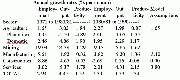 Table 5(v): Annual growth rates of employment, output and productivity 1971-1990
Source: Department of Census & Statistics (1976) Table 9;
Table 5(v): Annual growth rates of employment, output and productivity 1971-1990
Source: Department of Census & Statistics (1976) Table 9;
Department of Census & Statistics (1988) Table 13;
Department of Census & Statistics (1990) Table 2;
Central Bank of Ceylon, Annual Reports, 1982 and 1989.
As noted above, simulations for labour mobility were not performed nor were wage data not collected. The relative wages given are purely illustrative and were, in fact, drawn from another country. In future applications of the model it would be interesting to include relative wages for Sri Lanka and model them as they change in response to shortages and surpluses in the labour market. To do this would necessitate estimating the elasticity of wage response to unemployment rates and would then assume that relative wages only change in response to surpluses and shortages in the labour market. This would have to be investigated further before new modeling takes place.
3.4 The economy
The base data for the economic part of the model is displayed in Table 6. Destination investment series and incremental capital output ratios were estimated by Karunaratna for only three sectors - agriculture, industry and services. Thus the figures used for the eight economic sectors were based on the data for the three sectors but adjusted so as to simulate actual growth rates of the economy over 1986-1989. Karunaratna calculated two sets of figures for the ICOR - one lagged and one not - under the assumption that new investment was not immediately utilised. For the model his lagged values have been taken but the difference in application is small for either set of ICORs differing on average by only a few percent. His results are given in Table 7 and the figures retained in Table 6.
 Table 6(v): Base Data for Economy Model
Source: Economic data: 1989 Central Bank Report
Table 6(v): Base Data for Economy Model
Source: Economic data: 1989 Central Bank Report
Investment data: S.A. Karunaratna, 'Estimation of Overall and sectoral incremental capital output ratios of Sri Lanka', Seminar Paper No. 3/87, August '87, University of Colombo, Sri Lanka Association of Economists Seminar Paper Series.
 Table 7(v): Overall and Sector ICORs for certain sub-periods
Source: Karunaratna op.cit.
Table 7(v): Overall and Sector ICORs for certain sub-periods
Source: Karunaratna op.cit.
4. Results of the base scenario retained (scenario 1)
The base scenario was built upon the parameters described in the previous section. Results and graphs illustrating the results are lengthy and therefore only a few are produced.
Re-capping, population was 16.1mn in 1986, it had a life expectancy at birth of 72.2 years, it grew between 1986 and 1987 at the rate of 1.71% or 1.6% if international migrants were excluded. By the year 2000 the population is expected to reach 18.9mn of which 49.5% are expected to be females, life expectancy to be 73.5 years, natural population growth 1.1% and actual growth after subtracting international migration to be 0.8%. As noted above in section 3.1, these figures are similar for the year 2000 to the Government's own more detailed projections.
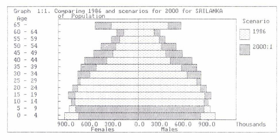
Graph 1.1 gives the population pyramid for 1986 and the year 2000 94 . It shows the aging of the population as fertility rates drop and life expectancy increases. Numbers for both females and males in the working ages 10 to 64 all grow over the period and the Graph 1.1 clearly shows that the sharp reduction in fertility did not, by the year 2000, have much impact in reducing the active population. There are 59.5% more women aged 64 and over in the year 2000 compared with 1986 while those aged 0-4 have reduced by 18.9% over the same time period. The same figures for men are 42.8% and 19.1% respectively.
Education results for the base scenario simulate the sharp decline from secondary to tertiary education, while the numbers in the penultimate year at secondary school (grade 11) rise significantly both in comparison to grade 10 and by the year 2000 compared with 1986. This picture reflects the desire of prospective 'A' level students to stay in school and repeat a year in order to improve their 'O' level results. Good 'O' and 'A'`level results are still the only way to enter university education and therefore qualify for higher paying jobs. A premium is put on university graduates by the fact that there are few places in university compared with the numbers in secondary school. Of particular note is the greater number of female students than male students in almost every grade. Nevertheless, the numbers of females in the pre-university grades 12 and 13 are expected to decline by the year 2000, a phenomenon also projected for males although not to the same extent if existing trends continue.
Economic results for the base scenario show the proportion of investment over GDP rising from 23.6% in 1986 to 28.4% by 2000 (illustrated in Graph 15.1 below). This gives rise to an overall GDP growth rate of 5.75% p.a. in 1986 rising to 6.80% by the year 2000. These growth rates are much higher than the GDP growth rates actually obtained over 1986-1990 which were 4.3%, 1.5%, 2.7% and 2.3% respectively 95 . In 1990, however, GDP rose by 6.2% and this has given confidence to MPPI staff that it will continue to rise at this rate to the year 2000. This might seem overly ambitious for a base scenario but reflects Government wishes, clearly the model can explore the implications of lower growth rates than this as will be seen in later scenarios. The main spurts to growth between 1986 and 2000 were anticipated to come from agriculture - to increase its growth upwards by 34.7 between 1986 and 2000 - and from construction - to increase its growth upwards by 24.8%. Thus by 2000 the most important economic sectors were anticipated to be agriculture, followed by trade, manufacturing, utilities and then construction.
The results for the labour market are given under the assumption that labour output coefficients reduce over time to reflect technical progress. Unsurprisingly, the lowest educated are found in agriculture while those with 'O' levels and more are found across all sectors particularly in manufacturing , trade and the public sector. It is projected that educated labour will be absorbed more in public administration than elsewhere.
For unemployment, overall unemployment at first rises from 14% in 1986 to 15.3% by 1989 before gradually falling as the high average 6 percent GDP growth rates bite by the year 2000. Note that these unemployment rates are calibrated to the results of the 1986/87 survey and represent the definition embodied therein. The model calculates the residual between labour supply and demand in terms of individuals not in terms of the number of hours worked. Therefore no insight into low productivity or low efficiency employment can be inferred nor can anything be said about underemployment. Nevertheless, despite the high growth rates assumed in the base scenario, unemployment in the Sri Lankan economy is only projected to fall by about 30% over 1986-2000. This is because of the increase in the labour force brought about by previous high labour force growth rates and the increase in labour supply due to the projected increasing desire to work of females.
The results of unemployment by education show unemployment falling slightly for those with incomplete primary education because demand rises faster than labour supply, the education system expands and also becomes more efficient by reducing the dropout rate for the lowly educated. Similarly, unemployment for incomplete secondary reduces by the year 2000. This phenomenon is reversed for the higher educated in both categories considered. In particular the expansion in higher education assumed in the base scenario leads to an almost doubling of this category in the labour supply from 339,000 to 713,000. Labour demand also sharply increases because of price, technology and the inflation of job requirement qualifications but not by enough to offset labour supply increases and thus educated unemployment for graduates rises in absolute numbers from 92,915 to 130,627 over 1986 to 2000. Nevertheless, the unemployment rate declines for this highest educated group from 27.4% in 1986 to 18.3% by 2000.
The last set of results for the base scenario, give the labour balances for occupations in 1986 and the year 2000. The results are not very interesting, as noted previously, because of the broad occupational categories chosen and, consequently, directly reflect the pattern of unemployment by level of education described in the paragraph above. Surpluses for all occupations come about for all levels of education. Given that there are no shortages for any occupational categories over the projection period the model could not show its versatility in substituting between occupations should one occupation be in surplus and another in deficit.
The base scenario is a reference scenario with which other scenarios can be compared. It is not meant to be a precise projection of what will happen, but it tries to give a best guess of where the Sri Lankan economy was heading over the future decade. Its power comes from being able to examine the results of 'what if' statements with the object of increasing our understanding of current and future events. The power of the approach also comes from the use of 'alternative' scenarios because the comparison of one scenario with another cancels out a some of the forecasting errors associated with point estimates. Then results are interpreted in terms of relative changes and the direction of change and not in absolute numbers. This is illustrated next when a number of alternative scenarios are examined.
5. Alternative scenarios
Six alternative scenarios were examined, the first was the base scenario discussed in the last section and five others that are discussed in this section. The six scenarios were:
Scenario 1: Base Scenario
Scenario 2: High growth from increased investment and foreign savings to meet full employment by the year 2000
Scenario 3: An Economist's interpretation of Scenario 2:
-
Increased outward international migration
-
Increased demand for educated labour
-
Increased participation rate for educated labour
-
Labour productivity increased by 10% across the board
-
Increased productivity of new investment
-
Higher growth from increased investment rate
-
Reduced school leaving and dropout rates
-
Changed retirement pattern to retain higher educated
Scenario 4: Scenario 3 plus changed pattern of investment toward manufacturing - an industrialisation or Newly Industrialised Country (NIC) pattern of growth and investment scenario
Scenario 5: Scenario 1 plus increased population growth
Scenario 6: Worst case scenario with constant investment (i.e. proportion of investment over GDP the same as 1986) and reductions in public employment.
The details of the quantitative parameter changes for all the six scenarios examined are not presented here nor are numerical results and only two graphs are given. This is because detailed results are too lengthy to report in full here.
5.1 High growth from increased investment (scenario 2)
In this scenario, the Government plans to raise economic growth significantly through attracting foreign savings and privatising the Sri Lankan economy. In 1991 investment as a proportion of GDP was 23% of which 13% arose from national savings and 10% from foreign savings 96 . This gave a 6% GDP growth rate in 1991. The Government anticipates raising investment to 30% of GDP over 1991-5 and to 33% over 1996 to 2000. It hopes that both domestic and foreign savings as a proportion of GDP will both rise by approximately 50% during the 1990s to achieve this. By the year 2000, under these conditions, growth is aimed to be averaging 9% a year (Table 8).
 Table 8(v): Required Growth Scenario 1991-2000
Source: Sri Lanka Economic Prospects for the 1990s (op.cit.)
Table 8(v): Required Growth Scenario 1991-2000
Source: Sri Lanka Economic Prospects for the 1990s (op.cit.)
When these investment assumptions are fed into the model, with no other changes, we see that overall growth of GDP (Table 9) rises from 5.8% a year to 8.4% by the year 2000 and unemployment falls from 15.1% in 1987 to nearly zero by the year 2000 i.e. the high investment and growth envisaged will lead to full employment by the year 2000. However, a closer examination of the results shows shortages for lower educated workers and unemployment for the higher educated. The growth and educational composition of labour supply is assumed, in scenario 2, to remain the same as in the base scenario. The increase in economic growth leads to increases in labour demand. Under the assumption of no change in the technology used to fuel the increase in economic growth then the scenario assumes the same composition of labour demand for labour by educational level as in the base scenario. Since unemployment is bigger for higher educated labour than the lower educated in the base scenario the net effect of increased growth is to erase unemployment for the lower educated, while making a dent in the higher educated unemployment rate but not eliminating it. An important conclusion here is that there is a danger that the Government's programme for new growth might be hampered by shortages in unskilled labour. This is similar to the situation then prevailing in Malaysia whose push for growth led to immigration of unskilled and largely illegal labour from Indonesia.
 Table 9(v): Projections of economy (Scenario 2)
Source: Model generated results.
Table 9(v): Projections of economy (Scenario 2)
Source: Model generated results.
5.2 An 'economist's' interpretation of scenario 2 (scenario 3)
How robust is the conclusion of the previous section that a push for growth could be hampered by unskilled labour shortages? This is the question addressed in Scenario 3. The main changes were:
Increased outward international migration. The rate was raised from .22% of the population to .30% to reflect the outward push due to continuing unemployment levels to the year 2000
Increased demand for educated labour. The coefficients in Variable 36, which is a matrix that allocates labour by education level to each economic sector, were altered across the board to simulate an increased demand for educated labour. This is likely to occur for a number of reasons. First, the growing numbers of the higher educated will lead to smaller wages on average making them more attractive to employers. Second, the faster growth assumed in this scenario will require newer technologies and higher skilled people to manage and operate them. Third, as the number of educated people increases there will be an inflation in job requirements as employers ask for higher and higher qualifications to screen job applicants.
-
Increased participation rate for educated labour. The labour force participation rates ten years hence i.e. Variable 42 for education levels three and four were increased slightly to simulate the increased desire to work, particularly for female graduates, as employment opportunities increase due to the increased demand for educated labour.
-
Labour productivity increased. Labour productivity in each economic sector, variable 45, was increased across the board by 10% to reflect the expected technical progress from increased foreign savings and investment.
-
Increased productivity of new investment. The elasticity of output with respect to capital was increased slightly (variable 46) to simulate the higher expected productivity of the new investment expected.
-
Higher investment rate. The same parameters were used, as in scenario 2, to increase the proportion of investment in the economy and the consequent higher growth over the base scenario. The combined effect of higher investment and higher efficiency of investment led to GDP growth of 9.1% a year by the year 2000 compared with 8.4% in scenario 2.
-
Reduced school leaving and dropout rates. The increase in demand for higher educated labour is likely to motivate students to stay in school and for the education system to become more efficient. Dropout rates (variable 23) and leaving rates (variable 24) for education levels three and four were therefore reduced a little.
-
Changed retirement pattern to keep higher educated. Slight changes in the retirement pattern by education level were made to reflect the increased demand for educated labour (variable 40). Thus a larger proportion of those with education levels one and two were assumed to retire, and a smaller proportion for levels three and four in comparison with the base run.

What was the net effect of these changes? First, as Graph 15.1 shows (the changes in value added by sector for each of the first three scenarios is given) the growth rate in scenario 3 is higher than in the preceding scenarios, but the same pattern of economic activity is preserved - agriculture and trade remain the two biggest activities in terms of value added, followed by manufacturing and utilities.
Labour demand reduces sharply for education levels one and two and, because supply reduces only slightly, the shortages for the lower educated turn into unemployment of 11.8% and 18.5% respectively. For education level three, despite a higher labour demand and reduced labour supply as more continue on into higher education, unemployment drops over scenarios 2 and 3 but still remains at the level of 11.8% of the labour force. The combined strategy has, nevertheless, succeeded in providing full employment among university graduates with unemployment falling to a frictional 1.4%. When adding up over all education levels, Graph 20.5 shows that unemployment has remained about the same in Scenario 2 but risen overall for Scenario 3 - thereby illustrating that higher growth rates do not necessarily mean lower unemployment when educational supply and demand levels are out of balance and when lower levels of education, quite obviously, cannot substitute for higher levels of education.

In conclusion the results of this scenario suggest that shortages of unskilled labour are not inevitable, as scenario 2 at first sight concluded, if the Government in combination with the technical progress expected expands and makes more efficient its education system when it makes its push for greatly increased growth. It may well be, and further experimentation within this scenario could explore these limits, that there will be shortages of skilled labour and not unskilled labour that the simpler analysis in scenario 2 foresaw.
5.3 A 'NIC 97 ' scenario - i.e. scenario 3 plus changed pattern of investment (scenario 4)
Scenario 4 is exactly the same as scenario 3 with the exception that the pattern of investment and, consequently, output is changed. This was to put a larger emphasis on manufacturing and less on trade and agriculture than in the previous scenarios. Such a pattern might be expected if a large push for growth is attempted as seen in other fast growing Asian nations 98 . What was done here was to reduce direct investment by 30% in agriculture and trade and re-allocate it to manufacturing. Financial sector investment was slightly increased to simulate the possible increased activity in that sector and investment in public administration was reduced to simulate further the increased privatisation likely from such a scenario.
Because manufacturing is more capital intensive than agriculture but not trade, labour demand reduces for all education levels and unemployment increases. The implications of changing strategy from agriculture to manufacturing therefore, without compensating measures, is higher unemployment.
5.4 Scenario 1 plus increased population growth (scenario 5)
The total fertility rate of females was raised by 10%. However, the effect on labour supply and therefore unemployment was negligible across all educational levels. Those who were born in 1986 only enter the labour force in 1996, assuming they do not stay on in school, and thus the effect is small. A longer time period of 22 years or more is required to allow the 1986 newly born to pass completely into the labour force. Excessive concern with reducing population growth in Sri Lanka thus seems unnecessary at least in terms of the labour market in the short to medium term. Indeed the converse problem of an aging population is showing and the need for a smaller number of younger workers to support a growing older population.
5.5 A worst case scenario (scenario 6)
In this scenario, investment as a proportion of GDP is assumed to be constant throughout the period 1986 to 2000. In addition the investment allocated to the public sector was halved reducing its growth rate by half and the investment released by this was allocated elsewhere to manufacturing. No other changes over and above the base scenario were made. The scenario is, perhaps, inaptly named since a respectable 5.6% real growth in GDP is maintained and, because of slowing population growth, per capita income growth rises from 4.0% a year in 1986 to 4.8% by 2000. In the base run GDP growth was assumed to rise at the rate of 5.8% a year in 1986 rising to 6.8% by the year 2000. The results of this scenario are predictable. The lower growth coupled with the redirection of investment from the public administration to manufacturing leads to a doubling of the higher educated numbers unemployed and overall unemployment rises from 9.9% in the base run to 19.3% in this 'worst case' scenario. It may be concluded, therefore, that if the Government's growth push fails to raise the growth rate of the economy from its historical rate of around 5% a year and privatisation leads to higher growth in manufacturing but a halving of employment in the public administration, then unemployment among the educated will rise rapidly. The social consequences of the Government's gamble failing are, therefore, serious.
6. Comparison of some key MACBETH variables (base scenario) with "actual" figure around 2000
Comparisons of some of the main variables projected in the MACBETH with "actual" values are given in Table 10. It is worth mentioning that it is very difficult to assess, from the international compendiums used, whether the definitions of the variables are the same. Population figures can be relied upon but economic data such as unemployment rate, employment by economic sector and investment require careful analysis of sources that is very difficult outside the country itself. So saying, it can be seen that the demographic projections of the model compare very well with actual values. Population growth, life expectancy at birth and total fertility rate are very close although there is some divergence when broken down by sex. The sex ratio in the model is a fixed variable and so, undoubtedly, this has not remained constant in the country with more males being born than females than was originally expected.
| Table 10(v): Comparison of some key MACBETH variables (Base Scenario) with 'actual' figures around 2000 |
| Variable |
|
1996 |
2000 |
MACBETH result in Year 2000 |
% difference between actual and projected |
| Population - total |
|
|
18826 |
18940 |
0.6 |
| Population - male |
|
|
9327 |
9559 |
2.5 |
| Population - female |
|
|
9498 |
9380 |
-1.2 |
| Population growth p.a. |
|
|
1.0 |
1.06 |
6.0 |
| Total Fertility Rate |
|
|
2.1 |
1.93 |
-8.1 |
| Life Expectancy at birth |
|
|
73.1 |
73.5 |
0.5 |
| Real GNP growth % p.a. 90-98 |
|
|
5 |
6.8 |
36.0 |
| Employment in Agric % |
|
35.1 |
|
47.7 |
35.9 |
| Employment in Industry % |
|
22.4 |
|
22.0 |
-1.8 |
| Employment in Services |
|
38.8 |
|
30.2 |
-22.2 |
| GDP in Agric % |
|
21.1 |
|
21.9 |
3.8 |
| GDP in Industry % |
|
27.5 |
|
41.9 |
52.4 |
| GDP in Services % |
|
51.4 |
|
36.1 |
-29.8 |
| Unemployment % |
|
|
11.3 |
10.0 |
-11.5 |
| Gross domestic investment/GDP % |
|
|
25.4 |
28.4 |
11.8 |
Sources: UNDP: Human Development Report 2000, (Oxford University Press, Oxford, 2000) and ILO: Key Indicators of the Labour Market, (ILO, Geneva, 1999)
Economic growth rate projections have a major impact on employment projections and , as can be seen, the growth in Sri Lanka was less than foreseen at 5% a year instead of the forecasted 6.8 - undoubtedly due to the ambitiously forecasted gross domestic investment rate of 28.4% being higher than the actual of 25.4%. The ambitious figure of 28.4% was the target of the Government at the time I did the projection, and was known to be ambitious but was what the Government wished to explore and therefore retained for the base scenario and most of the other scenarios. The structure of employment was significantly different (although we are comparing available data in 1996 with the projections for 2000) with less in agriculture and more in services projected by the model - this could well be due to differences in definition of sectors rather than actual differences but again only an in-depth analysis of the data on the ground could tell us that. Similarly, there are big differences in the allocation of GDP by sector with GDP in services under-estimated in the model, which led to the concomitant under-estimation of employment in services. Nevertheless, these major structural differences did not show up in the unemployment rate, which was roughly similar from, actual to projected at around 10%. However, the mismatch in the structure of employment would have led (data not available to show this) to significant differences in the demand for types of occupation with agricultural occupations more in demand than expected and service sector less in demand. This, in turn, would lead to a lower demand for educated labour and higher for unskilled.
Thus, what can be said about the utility of the model given its mixed forecasting performance? The main conclusion, as elsewhere, is that the model can be useful if data are both reliable and internally consistent. In the absence of such data reliable conclusions must depend on the realism of the scenario chosen. The high expectations of investment possibilities anticipated by the Government at the time the projections were done should have been tempered with more realism - this was also known at the time but illustrates that 'independent' forecasts would have served the Government better than accepting, at the time, too much false optimism about the Sri Lankan economy.
7. Summary and conclusions
7.1 On the model
1.The model performed well in the actual Sri Lankan situation as a tool to assist in the upgrading of skills (data analysis, micro-computer processing, presentation of results to management) of Sri Lankan social scientists engaged in human resource analytical issues. The model continues to be used in Sri Lanka for baseline projections and to assist in data consistency checks.
2. The model can provide insights into labour market analysis. It goes much further than a traditional 'manpower requirements' approach but, in its reduced form (i.e. without using the labour flexibility option), can imitate the manpower requirements approach and this is useful in providing baseline projections of manpower.
3. A number of policy issues of crucial concern to Sri Lanka may be examined with the model. This could be further enhanced through increasing its flexibility in a number of areas. Three main areas where improvements would be useful are:
Parameter changes. The model currently allows changes in a number of parameters that then impact on the major dynamics of the model. These can be entered in the base year and changed again after 10 years. Nevertheless, it would be desirable to be able to intervene in intermediate years as well even at the risk of complicating data entry into the model. This would then, for example, allow stochastic variables to be entered such as interruptions in agriculture production because of drought that occurs randomly in Sri Lanka but has short term devastating effects. The following variables need to be amenable to change in this way: total fertility rate, life expectancy, international migration, school repetition rates, school dropout rates, investment ratio over GDP, economic growth rates by economic sector, and the retirement of the labour force by education level.
Model changes. Three areas of possible improvements were considered - including an input-output structure, better specification of labour demand in the labour market and including wages. None of these changes present simple adaptations of the model. An input output structure could help in examining indirect effects of investment but would considerably complicate the model. It was thought better to introduce investment changes that had already taken account of indirect effects (see the description of the scenario where investment was changed). Second, although the current labour market specification is simple it can allow behavioural labour market mechanisms to be introduced through changes in exogenous inputs. On the other hand, not enough is known about labour market mechanisms in Sri Lanka to provide new model specifications and new research is required that examines the different labour market segments to increase understanding of the complexities involved. Third, wages are already included in the model, or rather relative wages since prices are exogenous to the model to give signals to labour movements between occupation levels and skills. This option was not used in the Sri Lanka application because of the problems of data. If one could estimate the elasticity of response of wages with respect to the labour balance between different workers with different educational levels changes., this would enhance the interest of the model. However, wage data is not available in Sri Lanka to allow this to be done.
Scenario analysis. The exogenous changes introduced for each of the six scenarios presented were introduced on a 'back of the envelope' basis. It would be desirable to put more work into alternative future scenario paths. For example, scenario 4 simulated a 'NIC' expansion path. The coefficients for investment, growth, education, technology etc. were guessed. However, data exist for these parameters for NIC and nearly NIC countries such as South Korea, Taiwan, Singapore, Hong Kong, Thailand and Malaysia. Some further research is required to obtain these coefficients which could then be relayed into a vastly improved 'NIC' scenario and re-run through the model.
7.2 On the economy
There is not much that can be said about training and occupation mismatches because the aggregation of data available from censuses and surveys are inappropriate, even to the extent of being useless for manpower analysis purposes. It would be desirable to have a data base that measured the skill level of workers that not only took into account their education, length of time working and occupation but also their quality. In the meantime it would be useful to re-calibrate the model with occupational classifications that identified critical skills or, if that concept proves to be elusive, something that can allow Sri Lanka to measure and develop its 'comparative advantage' in human resources.
There are major inconsistencies between available education data and the labour force. The numbers in school and leaving to join the labour force, as implied by Ministry of Education data (for school attendance, dropout, repetition and graduation rates) are inconsistent with the changing pattern of the labour force by level of education. It was not possible to judge whether the fault lay in the education or the labour force data. The inescapable conclusion is that the education statistics are incompatible with the labour force statistics. Clearly, consistency checks of flows of educated people by age and grade out of the education system are not matched with flows into the labour pool and labour force.
Population growth rate uncertainties (i.e. will it be higher or lower than trend) make very little difference to unemployment by the year 2000 simply because the newly born take up to 15 years to enter the labour force and with the gradually increasing length of education in Sri Lanka this period will be even longer than before.
Changing the pattern of investment away from agriculture toward more capital intensive sectors like manufacturing increases unemployment.
The high growth scenario aimed at, at that time, by the Government, will reduce unemployment but not totally eliminate it because a)there is a mismatch between type of educated supply and demand, b) new investment, although assumed more productive, is capital intensive in nature. It may well be, and further experimentation within this scenario could explore these limits, that there will be shortages of skilled labour and not unskilled labour if the Government's high growth strategy succeeds.
A worse case scenario whereby the Government's high growth strategy fails could lead to unemployment rates of the order of 19.3% by the year 2000 compared with the trend (in the base scenario) of 9.9%.
The comparison between 'actual' values of some key variables and the base scenario forecasts for the year 2000 showed mixed results. The demographic projections were excellent but the economic forecasts were too optimistic in terms of economic growth. The results do not question the validity of the model as much as its political context - a forecasting exercise is best done by an independent group that is allowed by the Government to have access to available data.
VII: Conclusions
Manpower planning
This monograph has re-examined the manpower planning debate in developing countries, presented a number of theories that have tried to explain the causes of mismatch on the labour market with emphasis on the main mismatch - that of unemployment. Next the monograph illustrated how difficult it has been to agree on definitions on exactly what is being measured in the labour market field. This was followed by the presentation of a model, the MACBETH model, that seeks to incorporate some of the main lacunae in manpower models to date. An application of the model to Sri Lanka then illustrated some of the strengths and weaknesses of the model. The penultimate chapter presented an alternative methodology that, as suggested in the literature, could provide a powerful alternative to simulation models of manpower forecasting.
In the first chapter it was argued that the use of models for manpower planning do still have a role to play. Labour market models are useful both for labour market analysis and to help to design labour market information systems. Normally, the argument goes, models cannot be built without an underlying labour market information system. But this is chicken and egg, and both are dependent on each other.
How to determine the future training needs of the labor market in developing countries is a question that has confronted manpower analysts and educational planners for decades. There is no easy solution simply because no-one can forecast the future and, therefore, what labor demands are likely anymore than one can predict stock market movements or future economic growth rates. This has not stopped people from trying. However, models to perform manpower analyses have been subject to such scathing criticism that manpower practitioners have shied away from modeling techniques and as such there is a gap to be filled. As now a combination of techniques under the general heading of "labour market signalling" have become the accepted methods, in recent years, to assess manpower needs. However, few countries have created a system to do this and there is much theorizing but little action.
One of the main objections to the manpower-forecasting methodology is that the elasticity of substitution between different kinds of labour is equal to (or near) zero. This is why the MACBETH model has a system to move labour between different levels of education and occupations. Although it is agreed that rigid adherence to manpower plans would be ludicrous the use of labour market information and labour market analysis to look at alternative scenarios of the labour market should not be dismissed. The dominant idea that no planning for human resources is warranted and that, instead of planning, all that needs to be done is to monitor the reactions and trends of the labour market, is rejected in the monograph. This is because to give guidance for present decisions, one needs what is never available: information on future earnings associated with different types of education. Data from the past are the best we can do, and reliable estimates of lifetime income streams are only available for those educated many years ago. The problem is that labor markets and the supply of educated persons to those markets can change so as to make past income streams poor predictors of future ones. Take the example of primary education. Rate of return analysis is used as a rationale for giving priority to it, for the rate of primary education is said to be typically higher than for secondary or higher education. But the calculation of rates is based on data for cohorts that received their schooling many years ago, when primary education was much less scarce than it is today.
The concern with manpower planning has led some authors to concentrate on the preparation and organisation of labour in Labour Market Information Systems (LMIS) as an 'alternative' to forecasting. Clearly, the mere collection of data sets without the sort of guide provided by a model is ridiculous. The publications are potentially useful, in a developing country context, to delineate the main variables of interest for manpower planning and to arrive at consistent definitions. Most of them do not do this. Indeed, at best they present a shopping list of items to be collected without providing an analytical framework within which to collect and then to analyze data for planning or policy formulation.
Manpower forecasting has been largely concerned, to date, with supply side policies and, in particular, implications for education and training. This is because the outcomes from the two main approaches to manpower forecasting, the manpower requirements approach (MRA) and the rate of return method (ROR), both concentrate on education and training policies. A growing response to the criticism of, particularly, these two methods has evolved into a generalised attack on the validity of any quantitative projections.
To counteract these criticisms, as far as possible, the MACBETH model presented in the monograph follows an heuristic approach. The results are presented in graphical form allowing a dialogue to be maintained with even the most numerically illiterate policy maker. The system is easy to use and to develop and relatively inexperienced professionals can be quickly trained to use the system. The system is heuristic because it produces results quickly, provokes discussion on the results emanating from the scenarios and leads the inquisitive into the search for new data sources, and better ways of understanding the labour market. The system can be used as a simple tool for continually monitoring what is happening in the labour market.
Labour market theories
Manpower planning has, at its core, the problem of mismatch between labour supply and demand i.e. unemployment. Consequently, a better understanding of the manpower planning problem can be helped by examining theories about the determination of unemployment. Therefore, the monograph set about, briefly, to overview some of the leading strands of thought that have attempted to explain, among other things, the economic causes of unemployment. Most theories do not centre on the causes of unemployment; rather they are mainly concerned with what causes, inter alia, accumulation, changes in the profit rate, inflation, growth, or changes in wages. Clearly, these causes are interrelated and so the emphasis of theory on a number of problems at once is not altogether surprising. The main conclusions of the chapter on theory were: first, it is inappropriate to examine labour markets in terms of equilibrium economics since there is no reason to presume that the forces that operate within labour markets interact more or less harmoniously and efficiently to grind out equilibrium levels of employment and associated working conditions. Second, labour markets are differentiated from one another, giving rise to empirically recognisable labour market segments or structures even though segmentation theory has tended to proceed in terms of divisions across the labour market as a whole and even though these divisions are perceived to be shifting and overlapping. Third, these labour market segments can be derived from 'horizontal' and 'vertical' factors. The former refers to determinants that prevail across all sectors of an economy, such as differentiation by gender and skill and the latter refers to the structuring within particular sectors of the economy. Fourth, with the rejection of equilibrium, it is necessary to demonstrate how labour market structures are socially reproduced, transformed or develop historically. This latter point does not mean degeneration into empiricism in which structure becomes identified mainly with large differences in behaviour as long as the structures are shown to incorporate underlying socioeconomic factors in an integral fashion. Fifth, labour market structures need to be derived from those socio-economic factors that arise out of the division between capital and labour and out of the profit imperative. This, in turn, implies a particular analytical and causal structure to labour market analysis, in which labour market structures are the reproduced and complex outcomes of the capital-output relation and its associated tendencies, such as productivity increase, deskilling, monopolisation etc. Finally, it does appear that the focus upon growth theory in recent years has led to questions of employment being more of an 'add-on' than a focus of economic theory per se, which differs sharply from the focus on the labour market by the classical economists and social reformers such as Keynes.
Data issues
Data availability for manpower or human resource planning at the national level are poor in developing countries. Further, there is much confusion over the meaning of employment and unemployment - and this is not confined to the developing countries with frequent changes of concepts and terminology occurring in the developed countries mainly to suit the interests of one political party or another. The manpower planner is often confronted with data which purport to measure underlying concepts but often have only a nod in the direction of precision. Not only are the methods that the manpower planner has to use severely criticised s(he) is also forced to walk on marshy ground as far as data are concerned. Nevertheless, the need for information about the future evolution of the labour force and occupations is there which is why, despite the poor quality of data and conceptualisation in the labour sphere, it is thought that the modeling of the manpower problem is a useful activity. It not only reveals alternative, albeit speculative, scenarios of the future it also reveals the underlying weakness of the data since a model forces data to be consistent and thereby reveals its main weaknesses.
The MACBETH model
MACBETH is, essentially, a recursive simulation model of the labour market and the evolution of occupational mismatches. The object has been to develop a model that was robust to data inconsistencies while being straightforward enough to be applied quickly in a developing country context. To date, data have not been available to calibrate the switching between occupations described in the last section. Nevertheless, the model has been used in many contexts and has been used as a pedagogic tool to introduce labour concepts into the manpower planing exercise. An example of its application was given for the case of Sri Lanka with the object to assess the implications of alternative growth paths on employment and (broad) skill requirements
The main conclusion, in Sri Lanka, was that the economic growth rate projections have a major impact on employment projections and, as was seen, the growth in Sri Lanka was less than foreseen at 5% a year instead of the forecasted 6.8 - undoubtedly due to the ambitiously forecasted gross domestic investment rate of 28.4% being higher than the actual of 25.4%. The ambitious figure of 28.4% was the target of the Government at the time and was known to be ambitious but was what the Government wished to explore and therefore retained for the base scenario and most of the other scenarios. The structure of employment was significantly different (although we are comparing available data in 1996 with the projections for 2000) with less in agriculture and more in services projected by the model - this could well be due to differences in definition of sectors rather than actual differences but again only an in-depth analysis of the data on the ground could tell us that. Similarly, there are big differences in the allocation of GDP by sector with GDP in services under-estimated in the model, which led to the concomitant under-estimation of employment in services. Nevertheless, these major structural differences did not show up in the unemployment rate, which was roughly similar with both actual data and the model projection giving an unemployment rate of around 10%. However, the mismatch in the structure of employment would have led (data not available to show this) to significant differences in the demand for types of occupation with agricultural occupations more in demand than expected and service sector less in demand. This, in turn, would lead to a lower demand for educated labour and higher for unskilled.
Thus the comparison between 'actual' values of some key variables and the base scenario forecasts for the year 2000 showed mixed results. The demographic projections were excellent but the economic forecasts were too optimistic in terms of economic growth. The results do not question the validity of the model as much as its political context - a forecasting exercise is best done by an independent group that is allowed by the Government to have access to available data.
What can be said about the utility of the model given its mixed forecasting performance? The main conclusion is that the model can be useful if data are both reliable and internally consistent. In the absence of such data reliable conclusions must depend on the realism of the scenario chosen. The high expectations of investment possibilities anticipated by the Government of Sri Lanka at the time the projections were done should have been tempered with more realism - this was also known at the time but illustrates that 'independent' forecasts would have served the Government better than accepting, at the time, too much false optimism about the Sri Lankan economy. The work on the model was carried out within the Ministry of Planning in Sri Lanka.
Thus, the model can provide insights into labour market analysis. It goes much further than a traditional 'manpower requirements' approach but, in its reduced form (i.e. without using the labour flexibility option), can imitate the manpower requirements approach and this is useful in providing baseline projections of manpower.
Labour market signalling
Labour market signaling is a useful adjunct to traditional forms of manpower analysis in that it advocates the need for wage and employment trends not only to guide schooling and training decisions but also to evaluate how well labour markets are functioning. The objective of signaling is that it can estimate whether there will be upward or downward pressure on the economic returns to investment in specific skills. Planners can monitor labor market conditions and evaluate training programs and can also focus upon skills that are of strategic importance to economic development and that take a long time to acquire.
The manpower planning school stresses labour market research and labour market signalling as 'the' alternative to manpower forecasting. There is no objection to the need for alternative techniques but, as also argued, there is a need to perform, and perfect, forecasting to provide a future vision to assist in the assessment of training and educational needs. The labour market signalling chapter showed that even with relatively detailed surveys, the identification of mismatches on the labour market and future training needs is not straightforward. The data collected in the surveys would help to calibrate some, but not all, parts of the MACBETH model.
Overall conclusion
The manpower forecasting debate was carried out vigorously in the 1970s and 1980s but appeared to end with the notion that all forecasting techniques that purported to assess manpower requirements in the future were dubious and that the future lay with labour market analysis and labour market signalling. In general, the monograph disputes the first notion but agrees that the, often over-simplified and non-flexible forecasting models of the past, should be supplemented with better data and improved labour market analysis.