1. Introduction
Medical physics can be one of the most challenging and rewarding applications of physics in society. Today, the diagnosis of a patient is rarely done without the use of imaging technology. Imaging allows us to peek inside the body, without resorting to invasive methods. Not only more comfortable and safe to the patient, imaging allows views of anatomy and physiology that cannot be obtained by any other means. Since the discovery of X-rays by Roentgen just before the dawn of the 20th century, the last 100 years have seen a veritable boom in medical imaging methods and technology. The original, time-honoured X-ray is one of the many methods in a radiologist's arsenal of imaging modalities. The physician can now examine the patient in a manner beyond imagination only 50 years ago.
The mathematical aspects of reconstruction techniques were first explored by the Austrian mathematician J Radon in 1917 who developed a general equation for the reconstruction of images from projections, also called the Radon transform. In 1922, several radiologists working independently devised the method for moving the tube over a patient, while the film beneath the patient was moved in the opposite direction. This method blurred all but one sharply focused plane of the target. This linear tomographic X-ray technique would remain the traditional method of obtaining three-dimensional information until the advent of Computed Tomography (CT). Hounsfield's invention of the CT scanner revealed to the public in 1972 was a major breakthrough in biomedical imaging. The result of X-ray CT is a two-dimensional map of the linear attenuation coefficient values (at some effective photon energy).
The first nuclear medicine imaging devices were developed in the late 1940s and early 1950s, where Geiger-Muller counters were used to measure counting rates from iodine-131 in the thyroid gland from point to point over the neck, and the numbers were written down in an equivalent array of points. The numbers alone were a poor display but lines of equal counting rate (isocount lines) were drawn which showed shape, size and relative uptakes of the two lobes and space-occupying lesions. The introduction of the Anger gamma camera in 1957 was the next dramatic change in imaging practice. Notwithstanding the low signal-to-noise ratio of the planar scintigrams obtained with a scintillation camera, a skilled and experienced human observer could visually interpret the images. The work of these pioneer radiologists progressed (unaware of Radon's publication) until 1961 when Oldendorf developed a crude apparatus for gamma ray transmission imaging with an 131I source. In 1963, Kuhl and Edwards developed an emission tomography system, and in 1966, a transmission system using _211Am with oscilloscope camera systems for data storage. In 1967, Anger implemented the concept of rotating gamma camera by rotating the patient at pre-defined angles in front of the detector. The image yields information about a location and concentration of a photon emitting radioisotope, which is administered to a patient. This technique is refereed as Single-Photon Emission Computed Tomography (SPECT).
The history of Positron Emission Tomography (PET) can be traced to the early 1950's, when workers in Boston first realised the medical imaging possibilities of a particular class of radioactive isotopes. Whereas most radioactive isotopes decay by release of gamma rays and electrons, some decay by the release of a positron. A positron can be thought of as a positive electron. Widespread interest and an acceleration in PET technology was stimulated by development of reconstruction algorithms associated with X-ray CT and improvements in nuclear detector technologies. By the mid-1980s, PET had become a tool for medical diagnosis for dynamic studies of human metabolism and for studies of brain activation.
It is believed that after X-ray radiology, the use of ultrasound in medical diagnosis is the second most frequent investigative imaging technique. The earliest attempts to make use of ultrasound date from the late 1930s; ultrasonic imaging based on the pulse-echo principle became possible after the development of fast electronic pulse technology during the second world war. However, it was not until 1958 that the prototype of the first commercial two-dimensional ultrasonic scanner was described by Donald and was used to carry out the first investigations of the pregnant abdomen. Nuclear Magnetic Resonance (NRM) was invented in the mid 1940s; for this invention Bloch and Purcell were awarded a Nobel prize in 1952. Clinical NMR imaging, which burst on the world in 1980, now misguidedly known as MRI, is a form of tomography which results from imaging data obtained in quantitative form. The NMR signal intensity is related to the proton spin population in the imaging voxel which is detected by the NMR process, but it is modified by the amount of spin-lattice relaxation (T1) and the spin-spin relaxation (T2) of the protons which have occurred during the timings of the NMR pulse sequence used.
1.1 Medical imaging techniques
 Fig. 1.1. : Transaxial slice of the human brain (top) acquired with different imaging modalities (bottom) from left to right: X-ray CT, MRI, SPECT and PET
In general, imaging can address two issues: structure and function. One can either view structures in the body and image anatomy or view chemical processes and image biochemistry. Structural imaging techniques can image anatomy and include ultrasound, X-rays, CT and MRI. One can distinguish bone from soft tissue in X-ray imaging. Organs become delineated in CT and MRI imaging. Biochemical modalities differ from structural ones in that they follow actual chemical substituents and trace their routes through the body. These methods give functional images of blood flow and metabolism essential to diagnoses and to research on the brain, heart, liver, kidneys, bone, and other organs of the human body. Since usually anatomical structures serve different functions and embody different biochemical processes, to some degree biochemical imaging can give anatomical information. However, the strength of these methods is to distinguish tissue according to metabolism, not structure.
As an example, Fig. 1.1 shows a transaxial slice through the human brain (top row) acquired with different imaging modalities (bottom row) giving different information about the brain function and anatomy. Several clinical applications are associated to each imaging technique.
1.2 Positron Emission Tomography in medical imaging
Positron emission tomography (PET) is a well-established imaging modality which provides physicians with information about the body's chemistry not available through any other procedure. Three-dimensional (3D) PET provides qualitative and quantitative information about the volume distribution of biologically significant radiotracers after injection into the human body. Unlike X-ray CT or MRI, which look at anatomy or body morphology, PET studies metabolic activity or body function. PET has been used primarily in cardiology, neurology, and oncology.
Within the spectrum of medical imaging, sensitivity ranges from the detection of millimolar concentrations in MRI to picomolar concentrations in PET: a 109 difference (Jones 1996). With respect to specificity, the range is from detecting tissue density and water content to a clearly identified molecule labelled with a radioactive form of one of its natural constituent elements. This sensitivity is a prerequisite if studies are to be undertaken of pathways and binding sites which function at less than the micromolar level, and to avoid the pharmacological effects of administering a labelled molecule to study its inherent biodistribution.
The sensitivity of in vivo tracer studies is developed per excellence with PET, which is based on electronic collimation and thereby offering a wide acceptance angle for detecting emitted annihilation photons. Consequently, the sensitivity of PET per disintegration with comparable axial fields of view, is two orders of magnitude greater than that of SPECT cameras. A further sensitivity advantage for detecting low molecular concentration arises in PET when detecting molecules labelled with short-lived radioisotopes. With respect to imaging of molecular pathways and interactions, the specificity of PET arises due to the use of radioisotopes such as 18F and, to a lesser extent, 11C to label biochemical/physiological and pharmaceutical molecules within a radioactive form of one of its natural constituent elements. SPECT's ability to image some chemical processes is hindered by the fact that the isotopes are relatively large atoms and cannot be used to label some compounds due to steric reasons.
There is no doubt that PET has a long-term future in the study of receptors, neurotransmitters, drug binding and general pharmacology. In addition, it clearly still has unique roles in biochemistry/metabolism and physiology. With regards to research, the emphasis is to use PET to gain new information on disease processes, to assess the efficacy and mechanisms of therapy and to help drug development and discovery. Deriving new information on brain disease is the focus of many neuroscience research programmes based on PET, with an ever-increasing interest in the psychiatric area. Disease staging and assessment of therapeutic mechanism and efficacy are emerging not only for the brain but also in cardiology and oncology.
1.3 The aim of this work
The aim of this project is to develop a versatile Monte Carlo simulation environment and a reconstruction library taking advantage of modern software development technology and parallel computing technology and to use the simulation package as a development and evaluation tool for scatter correction methods and image reconstruction algorithms in 3D PET. This work was part of the PARAPET (PARAllel PET Scan) project, funded by the European Commission and the Swiss Government, which focused on the development of improved iterative methods for volume reconstruction of PET data through the use of high performance parallel computing technology. This project also includes the development of procedures and software for evaluation of a library of simulated, experimental phantom and clinical data.
The project involves leading players from the UK: the Hammersmith Hospital and Brunel University; Italy: the Ospedale San Rafaele, Milan; Switzerland: Geneva University Hospital; Israel: Israel Institute of Technology, Haifa; the scanner manufacturer ELGEMS, Israel, and the leading European supplier of embedded parallel processing hardware: Parsytec, Germany. The project has a strong European dimension bringing together leading researchers and clinicians and a leading hardware vendor and scanner manufacturer from across the European Union in a collaboration strengthened by the participation of peer organisations in Switzerland and Israel.
In addition to the Monte Carlo simulation package, the project will produce a package of analytical and iterative reconstruction algorithms for 3D PET imaging and make them available for clinical environments. A major aim of the project is to create parallel versions of these algorithms to run on distributed memory multiprocessor machines. The partners in the project use Parsytec CC series of machines, the main goal, however, is to create parallel software tools that achieve:
-
speed-up on the basis of elapsed wall-clock time;
-
scale-up in terms of progressively larger data sets as found on a range of scanners;
-
platform independence, thus running on clusters of high-end PCs and other distributed memory multiprocessor hardware architectures.
The following paragraphs will summarise the contents of this thesis :
-
An object-oriented library for 3D PET reconstruction has been developed (Labbé et al 1999a, Labbé et al 1999b). This library has been designed so that it can be used for many algorithms and scanner geometries. Its flexibility, portability and modular design have helped greatly to develop new iterative algorithms (Ben Tal et al 1999, Jacobson et al 1999) and to compare iterative and analytic methods in different clinical situations, and to parallelise the reconstruction algorithms.
-
The methodological basis for the Monte Carlo method is derived and a critical review of their areas of application in nuclear medical imaging is presented and illustrated with examples of some useful features of such sophisticated tools in connection with common computing facilities and more powerful multiple-processor parallel processing systems (Zaidi 1999a).
-
A Monte Carlo software package, Eidolon, has been developed which accurately simulates volume imaging PET tomographs. The code has been designed to evaluate PET studies of both simple shape-based phantom geometries and more complex non-homogeneous anthropomorphic phantoms (Zaidi et al 1997a, Zaidi et al 1999a). The package is well documented (Zaidi et al 1997b) and has been in the public domain since September 1999.
-
The Eidolon software package was successfully ported on a parallel architecture based on PowerPC 604 processors running under AIX 4.1. A parallelisation paradigm independent of the chosen parallel architecture was used in this work. A linear decrease of the computing time was achieved with the number of computing nodes (Zaidi et al 1998).
-
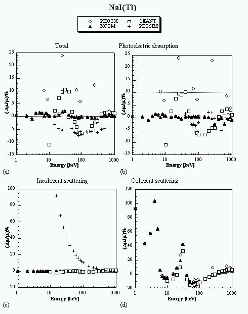
A comparison between different photon cross section libraries and parametrizations implemented in Monte Carlo simulation packages developed for positron emission tomography and the most recent Evaluated Photon Data Library (EPDL97) developed by the Lawrence Livermore National Laboratory (LLNL) in collaboration with NIST was performed for several human tissues and common detector materials for energies from 1 keV to 1 MeV. This latter library is thought to be more accurate and was carefully designed in the form of look-up tables and integrated in our simulation environment significantly improving the efficiency of the Eidolon simulation package (Zaidi et al 1999c, Zaidi 1999d).
-
An evaluation of common scatter correction techniques has shown that an accurate modelling of the scatter component in the projection data is necessary to estimate for an accurate scatter correction. An improvement and extension to whole-body 3D imaging of a recently proposed Monte Carlo-based scatter correction method (Levin et al 1995) and a new approach called Statistical Reconstruction Based Scatter Correction (SRBSC) based on estimating the low frequency component corresponding to scatter events using OSEM are proposed in this work (Zaidi 1999e) and evaluated against more common correction methods (Zaidi 1999f).
In chapter 2, the physical principles, basic features and performance parameters of PET are outlined, and some of the practical issues involved in obtaining quantitative data discussed. In chapter 3, the problem of image reconstruction from projections is defined in the context of 2D and 3D PET. Various analytical, rebinning and iterative algorithms proposed for 3D PET reconstruction are then reviewed and some innovative approaches resulting from the PARAPET project and their software implementations presented. As the implementation of 3D type reconstruction algorithms is time-consuming, issues in parallelisation and scalability are also discussed with the aim to reduce the effect of the time factor in practice and make 3D PET more generally accessible and clinically acceptable. In chapter 4, the derivation and methodological basis for the Monte Carlo method is presented and followed by an overview of existing simulation programs and a critical review of their areas of application in PET imaging. In chapter 5, the development, validation and main features of an object-oriented Monte Carlo simulator for 3D PET, Eidolon, is described in detail. A fast implementation of the program on a MIMD parallel architecture and the improvement of its efficiency and accuracy through the implementation of an up-to-date photon cross section library are then presented in Chapter 6. In Chapter 7, issues in scatter modelling and correction techniques in 3D PET are discussed and two new approaches presented. The characteristics and evaluation of these approaches against common scatter correction techniques is also presented using phantom simulations, experimental phantoms and clinical studies. Finally, key conclusions and suggested continuation of this research are presented in chapter 8.
2. Positron Emission Tomography : Physics and Instrumentation
The key advantage of PET is added sensitivity which is obtained by naturally collimating the annihilation photons through a physical process, without the use of absorbing collimators. As does SPECT, PET uses tracers but, these are labelled with positron emitting isotopes, such as Fluorine-18 (18F) and Carbon-11 (11C). PET tracers possess key advantages over SPECT tracers. They have a relatively short half-life which reduces the time of exposure to the patient and thus the absorbed dose. In addition, because 18F is similar in size to hydrogen, it can be used to replace hydrogen in biologically active compounds without altering their function. This opens up an entire group of metabolites which could not be labelled for SPECT. The major drawback is that a short half-life puts a practical upper limit on the activity of the manufactured isotope. A nearby or on-site cyclotron facility is therefore required. Many of the present design objectives of positron imaging tomographs focus on meeting the needs of brain imaging in neurology and of whole-body imaging in oncology. This section describes the physical principles underlying PET and discusses some of the instrinsic advantages that PET exhibits over SPECT imaging.
2.1 The physical principles of PET
In PET, pairs of 511 keV photons arising from electron-positron annihilations are detected in coincidence and allow to measure the concentration of a positron-emitting radionuclide. After intravenous injection of the positron-emitting radiopharmaceutical, patients are generally refereed to waiting rooms to allow its concentration in the tissue or organ of interest. Block detectors surrounding the patient are then used to detect the emerging annihilation photons.
A positron emission tomograph consists a set of detectors usually arranged in adjacent rings that surround the field-of-view (FOV) in order to image the spatial distribution of a positron emitting radiopharmaceutical (Fig. 2.1). After being sorted into parallel projections, the lines of response (LORs) defined by the coincidence channels are used to reconstruct the three-dimensional (3D) distribution of the positron-emitter tracer within the patient. An event is registered if both crystals detect an annihilation photon within a fixed coincidence time window depending on the timing properties of the scintillator (of the order of 10 ns for Bismuth germanate or BGO). A pair of detectors is sensitive only to events occurring in the tube of response joining the two detectors, thereby registering direction information (electronic collimation). There are many advantages associated to coincidence detection compared to single-photon detection devices: electronic collimation eliminates the need for physical collimation, thereby significantly increasing sensitivity and improving the spatial resolution. Accurate corrections for the background and physical effects are, however, essential to allow absolute measurements of tissue tracer concentration to be made.
 Fig. 2.1. : Originating from the decay of the radionuclide, a positron travels a few millimetres before it annihilates with a nearby atomic electron, producing two 511 keV photons emitted in opposite directions
A positron emission tomograph consists a set of detectors usually arranged in adjacent rings surrounding the FOV. Pairs of annihilation photons are detected in coincidence. The size of the transaxial FOV is defined by the number of opposite detectors in coincidence.
2.1.1 Positron emission and annihilation
Proton-rich isotopes may decay via positron emission, where a proton in the nucleus decays to a neutron, a positron and a neutrino. The daughter isotope has an atomic number one less than the parent. Examples of isotopes which undergo decay via positron emission are shown in table 2.1.
As positrons travel through human tissues, they give up their kinetic energy mainly by Coulomb interactions with electrons. As the rest mass of the positron is the same as that of the electron, positrons may undergo large deviations in direction with each Coulomb interaction, and they follow a tortuous path through the tissue as they give up their kinetic energy (Fig. 2.2).
| Table. 2.1. : Physical characteristics and production method of commonly used positron emitting radioiosotopes |
| Radioisotope |
Half-life (min) |
Maximum positron energy (MeV) |
Positron range in water (FWHM in mm) |
Production method |
| 11C |
20.3 |
0.96 |
0.28 |
cyclotron |
| 13N |
9.97 |
1.19 |
0.35 |
cyclotron |
| 15O |
2.03 |
1.70 |
1.22 |
cyclotron |
| 18F |
109.8 |
0.64 |
0.22 |
cyclotron |
| 68Ga |
67.8 |
1.89 |
1.35 |
generator |
| 82Rb |
1.26 |
3.35 |
2.60 |
generator |
When positrons reach thermal energies, they start to interact with electrons either by annihilation, producing two 511 keV photons which are anti-parallel in the positron's frame, or by the formation of a hydrogen-like orbiting couple called positronium. In its ground-state, positronium has two forms: ortho-positronium, where the spins of the electron and positron are parallel, and para-positronium, where the spins are anti-parallel. Para-positronium again decays by self-annihilation, generating two anti-parallel 511 keV photons. Ortho-positronium self-annihilates by the emission of three photons. Both forms are susceptible to the "pick-off" process where the positron annihilates with another electron. Free annihilation and the pick-off process are responsible for over 80% of the decay events. Variations in the momentum of the interacting particles involved in free annihilation and pick-off result in an angular uncertainty in the direction of the 511 keV photons of around 4 mrad in the observer's frame (Rickey et al 1992). In a PET tomograph of diameter 100 cm and active transaxial FOV of 60 cm, this results in a positional inaccuracy of 2-3 mm. The finite positron range and the non-collinearity of the annihilation photons give rise to an inherent positional inaccuracy not present on conventional single-photon emission techniques. However, other characteristics of PET which are discussed below more than offset this disadvantage.
 Fig. 2.2. : Schematic representation of positron emission and annihilation
2.1.2 Positron emitting radiopharmaceuticals
Nuclear medicine imaging involves studies of the localisation of administered radiopharmaceuticals by detection of the radiation emitted by the radionuclides. The radiopharmaceuticals can be administered to the patient by injection, orally or by inhalation. A radiopharmaceutical consists of a radionuclide with suitable radiation characteristics which is usually 'labelled' in a chemical reaction to a carrier. When labelled to a carrier, the main interest is the physiological and biological behaviour of the carrier and the radionuclide serves only as a tracer. There are several advantages of using radionuclides as tracers for in vivo studies. The physiological behaviour and the metabolism in different organs can be studied rather than the morphological structure. Important objectives such as the detection of lesions can be realised. However, since in most disease processes physiological or metabolic changes precedes changes in anatomy, nuclear medicine has a capability to provide earlier diagnosis.
While PET was originally used as a research tool, in recent years it come to have an increasingly important clinical role. The largest area of clinical use of PET is in oncology where the most widely used tracer is 18F-fluoro-deoxy-glucose (18F-FDG). This radiopharmaceutical is relatively easy to synthesise with a high radiochemical yield. It also follows a similar metabolic pathway to glucose in vivo, except that it is not metabolised to CO2 and water, but remains trapped within tissue. This makes it well suited to use as a glucose uptake tracer. This is of interest in oncology because proliferating cancer cells have a higher than average rate of glucose metabolism. 11C-methionine is also used in oncology, where it acts as a marker for protein synthesis.
PET has applications in cardiology, where 11N-NH3 is used as a tracer for myocardial perfusion. When 13N-NH3 and 18F-FDG scans of the same patient are interpreted together, PET can be used to distinguish between viable and non-viable tissue in poorly perfused areas of the heart. Such information can be extremely valuable in identifying candidates for coronary by-pass surgery. PET has been used in neurology in a wide range of conditions, and in particular in severe focal epilepsy, where it may be used to compliment magnetic resonance imaging. Another reason for the importance of PET lies in the fact that, unlike conventional radiotracer techniques, it offers the possibility of quantitative measurements of biochemical and physiological processes in vivo. This is important in both research and clinical applications. For example, it has been shown that semi-quantitative measurements of FDG uptake in tumours can be useful in the grading of disease (Hoh et al 1997). By modelling the kinetics of tracers in vivo, it is also possible to obtain quantitative values of physiological parameters such as myocardial blood-flow in ml/min/g or FDG uptake in mmol/min/g providing the acquired data is an accurate measure of tracer concentration. Absolute values of myocardial blood flow can be useful in, for example, the identification of triple-vessel coronary artery disease and absolute values of FDG uptake can be useful in studies of cerebral metabolism. Some examples of radiopharmaceuticals used in PET are shown in table 2.2, together with some typical clinical and research applications.
Prospects for the further development of several agents currently being investigated have been improved, and a number of established clinical procedures have developed an increased potential with the added application of the PET modality. These complementary roles of PET all contribute to an increased accuracy in nuclear medicine investigations.
| Table 2.2. : Examples of positron-emitting radiopharmaceuticals used in clinical PET studies with some representative investigations where quantification is of interest |
| Radioisotope |
Tracer compound |
Physiological process |
Clinical application |
| |
methionine |
protein synthesis |
oncology |
| 11C |
flumazenil |
bezodiazepine receptor antagonist |
epilepsy |
| |
raclopride |
D2 receptor agonist |
movement disorders |
| 13N |
ammonia |
blood perfusion |
myocardial perfusion |
| 15O |
carbon dioxide
water |
blood perfusion
blood perfusion |
brain activation studies
brain activation studies |
| |
Fluoro-deoxy-glucose |
glucose metabolism |
cardiology, neurology, oncology |
| 18F |
Fluoride ion
Fluoro-mizonidazole |
bone metabolism
hypoxia |
oncology
oncology - response to therapy |
2.1.3 Interaction of photons with matter
When electromagnetic radiation passes through matter, some photons will be totally absorbed, some will penetrate the matter without interaction and some will be scattered in different directions, with and without loosing energy. Unlike charged particles, a well-collimated beam of photons shows a truly exponential absorption in matter. This is because photons are absorbed or scattered in a single event. That is, those collimated photons which penetrate the absorber have had no interaction, while the ones absorbed have been eliminated from the beam in a single event. For the energies of interest in nuclear medicine imaging, a photon interacts with the surrounding matter by four main interaction processes. The probability for each process depends on the photon energy, E, and the atomic number, Z, of the material.
2.1.3.1 Photoelectric absorption
When a photoelectric interaction occurs, the energy of a photon is completely transferred to an atomic electron. The electron may thus gain sufficient kinetic energy to be ejected from the electron shell. The energy of the incoming photon must, however, be higher than the binding energy for the electron. Because the entire atom participates, the photoelectric process may be visualised as an interaction of the primary photon with the atomic electron cloud in which the entire photon energy E is absorbed and an electron (usually K or L) is ejected from the atom with an energy :
 |
(2.1) |
where Te is the binding energy of the ejected electron. A photoelectric interaction results in a vacancy in the atomic electron shell which, however, will be rapidly filled by an electron from one of the outer electron shells. The difference in binding energy between the two electron shells can be emitted either as a characteristic X-ray photon or as one or several Auger electrons. The relative probability for the emission of characteristic X-ray photons is given by the fluorescence yield . Characteristic X-ray emission is more probable for high Z materials.
The cross section for a photoelectric interaction depends strongly on the photon energy and the atomic number of the material and can be described approximately by :
 |
(2.2) |
2.1.3.2 Incoherent (Compton) scattering
In this process, the photon interacts with an atomic electron and is scattered through an angle q relative to its incoming direction. Only a fraction of the photon energy is transferred to the electron. After incoherent (or Compton) scattering, the scattered photon energy Es is given by
 |
(2.3) |
where mo is the rest mass energy of the electron and c is the speed of light. Equation (2.3) is derived on the assumption that an elastic collision occurs between the photon and the electron, and that the electron is initially free and at rest. It is evident from Eq. (2.3) that the maximum energy transfer takes place when the photon is back-scattered 180° relative to its incoming direction and that the relative energy transfer from the photon to the electron increases for increasing photon energies. The expression (2.3) is plotted in Fig. 2.3 for 511 keV photons and illustrate that rather large angular deviations occur for a relatively small energy loss.
 Fig. 2.3. : The residual energy of a 511 keV photon after Compton scattering through a given angle
The differential cross section per electron for an incoherent scattering for unpolarised photons, derived by Klein and Nishina (1927), can be calculated from
 |
(2.4) |
where re is the classical radius of the electron, and is given by
 |
(2.5) |
Equation (2.4) has been derived assuming that the interacting electron is free and at rest. The differential cross section per atom can be calculated by multiplying the Klein-Nishina cross section by the number of electrons Z in order to take into account the fact that atomic electrons are energetically bound to the nucleus. The Klein-Nishina cross section per electron should be multiplied by the incoherent scattering function S(x,Z), i.e.
 |
(2.6) |
where  is the momentum transfer parameter and l is the photon wavelength. For high-energy photons, the function S(x,Z) approaches the atomic number Z and the cross section will thus approach the Klein-Nishina cross section.
2.1.3.3 Coherent (Rayleigh) scattering
In coherent (Rayleigh) scattering the photon interacts with the whole atom, in contrast to incoherent scattering in which the photon interacts only with an atomic electron. The transfer of energy to the atom can be neglected due to the large rest mass of the nucleus. Coherent scattering therefore results only in a small change in the direction of the photon since the momentum change is so small.
The differential cross section per atom is given by the classical Thompson cross section per electron multiplied by the square of the atomic form factor F(x,Z)
 |
(2.7) |
where q is the polar angle through which the photon is scattered. The form factor will approach the atomic number Z for interactions involving small changes in the direction of the photon and for low photon energies. The form factor decreases with increasing scattering angle. The angular distribution of coherently scattered photons is thus peaked in the forward direction.
2.1.3.4 Pair production
If the energy of the incoming photon is greater than 1.022 MeV (two electron rest masses), there will be a finite probability for the photon to interact with the nucleus and to be converted into an electron-positron pair. The electron and the positron will have a certain kinetic energy and interact by inelastic collisions with the surrounding atoms. The cross section spair is proportional to the square of the atomic number Z. This type of interaction is not important for the photon energies commonly used in nuclear medicine.
 |
(2.8) |
2.1.3.5 The linear attenuation coefficient
When a photon passes through matter, any of the four interaction processes described above may occur. The probability for each process will be proportional to the differential cross section per atom. The probability of a photon traversing a given amount of absorber without any kind of interaction is just the product of the probabilities of survival for each particular type of interaction, and is proportional to the total linear attenuation coefficient, which is given by :
 |
(2.9) |
This attenuation coefficient is a measure of the number of primary photons which have had interactions. It is to be distinguished sharply from the absorption coefficient, which is always a smaller quantity measuring the energy absorbed by the medium. The mass attenuation coefficient is defined as the linear attenuation coefficient divided by the density r of the absorber. The attenuation of an incoming narrow-beam of photons when passing through a non-homogeneous object can be described by
 |
(2.10) |
where F is the photon fluence measured after the attenuator, Fo is the photon fluence measured without the attenuator and d is the thickness of the attenuator. Linear attenuation coefficients are often referred to as "narrow-beam" or "broad-beam" depending on whether they contain scattered transmission photons or not. Fig. 2.4. illustrates this concept with a simple single detector system measuring uncollimated and collimated photon sources. Narrow-beam transmission measurements are ideally required for accurate attenuation correction in PET. This is of course, determined by the geometry of the transmission data acquisition system.
 Fig. 2.4. : Schematic illustration of the concept of narrow-beam and broad-beam attenuation for a simple single detector system
In the broad-beam case (top), the source is uncollimated and this results in the deviation of some photons back into the acceptance angle of the collimated detector. Due to the acceptance of scattered events, the count rate will be higher in the broad-beam case, the effect of which is to lower the effective linear attenuation coefficient value. In the narrow-beam case (bottom), most scattered photons will not be detected. This is due mainly to the collimation of both the source and the detector. The difference between detected counts with and without the object in place is due to both total attenuation within the object and scattering out of the line of sight of the detector
2.1.4 Types of coincidence events
Coincidence events in PET fall into 4 categories: trues, scattered, randoms and multiples. Fig. 2.5. illustrates the detection of first three of these different types of coincidences.
 Fig. 2.5. : Types of detected coincidence events in PET
True coincidences occur when both photons from an annihilation event are registered by detectors in coincidence, neither photon undergoes any form of interaction prior to detection, and no other event is detected within the coincidence time-window.
A scattered coincidence is one in which at least one of the detected photons has undergone at least one Compton scattering event prior to detection. Since the direction of the photon is changed during the Compton scattering process, it is highly likely that the resulting coincidence event will be assigned to the wrong LOR. Scattered coincidences add a background to the true coincidence distribution which changes slowly with position, decreasing contrast and causing the isotope concentrations to be overestimated. They also add statistical noise to the signal. The number of scattered events depends on the volume and attenuation characteristics of the object being imaged, and on the geometry of the tomograph. Basically, we can distinguish single scattered events when one or both annihilation photons undergo one scattering and multiple scattered events where one of the two photons undergo two or more scatterings.
Random (or false) coincidences occur when two uncorrelated photons not arising from the same annihilation event are incident on the detectors within the coincidence time window of the system. The number of random coincidences in a given LOR is closely related to the rate of single events measured by the detectors joined by that LOR and the rate of random coincidences increase roughly with the square of the activity in the FOV. As with scattered events, the number of random coincidences detected also depends on the volume and attenuation characteristics of the object being imaged, and on the geometry of the tomograph. The distribution of random coincidences is fairly uniform across the FOV, and will cause isotope concentrations to be overestimated if not corrected for. Random coincidences also add statistical noise to the data.
A simple expression relating the number of random coincidences assigned to an LOR to the number of single events incident on the relevant detectors can be derived as follows. Let us define t as the coincidence resolving time of the system, such that any events detected with a time difference of less than t are considered to be coincident. Let r1 be the singles rate on detector channel 1. Then in one second, the total time-window during which coincidences will be recorded is 2t r1. If the singles rate on detector channel 2 is r2, then the number of random coincidences R12 assigned to the LOR joining detectors 1 and 2 is given by :
 |
(2.11) |
This relation is true provided that the singles rate is much larger than the rate of coincidence events, and that the singles rates are small compared to the reciprocal of the coincidence resolving time t, so that dead-time effects can be ignored.
Multiple coincidences occur when more than two photons are detected in different detectors within the coincidence resolving time. In this situation, it is not possible to determine the LOR to which the event should be assigned, and the event is rejected. Multiple events can also cause event mis-positioning.
2.2 Design configurations of PET tomographs
There has been a significant evolution in PET instrumentation from a single ring of bismuth germanate (BGO) detectors with a spatial resolution of 15 mm (Keller and Lupton 1983), to multiple rings of small BGO crystals resulting in a spatial resolution of about 5-6 mm (Phelps and Cherry 1998). Improvements in spatial resolution have been achieved by the use of smaller crystals and the efficient use of photomultiplier tubes (PMT's) and Anger logic-based position readout.
The most successful tomograph design represents a reasonable compromise between maximising system sensitivity while keeping detector dead-time and corruption from scattered and random coincidences at a reasonable level (Bailey et al 1997a). In particular, this performance has been achieved through the development of multi-ring tomographs equipped with collimators (or septa) between the detector rings. Coincidences are allowed only within a ring or between adjacent rings. The consequence of this is a considerable decrease in the sensitivity of the system, and the less than optimal use of electronic collimation, one of the main advantages of coincidence detection. By removing the septa and allowing acceptance of coincidences between detectors in any two rings of the tomograph, an increase in sensitivity by a factor of 4-5 has been achieved (Dahlbom et al 1989). Septaless tomographs can also be operated more effectively with lower activity levels in the field-of-view. Fig. 2.6 illustrates possible geometric designs of positron imaging systems.
An important consequence of the cost- and performance-conscious environments of health care today is the constant pressure to minimise the cost of PET tomographs by reducing the geometry from a full ring to a dual-headed device, while at the same time there is also pressure to provide the most accurate diagnostic answers through the highest performance possible. The dilemma is that both approaches can lower the cost of health care. Continuous efforts to integrate recent research findings for the design of both geometries of PET scanners have become the goal of both the academic community and nuclear medicine industry. The most important aspect related to the outcome of research performed in the field is the improvement of the cost/performance optimisation of clinical PET systems.
Dedicated full-ring PET tomographs have evolved through at least 4 generations since the design of the first PET scanner in the mid 1970s (Hoffman et al 1976) and are still considered the high-end devices. The better performance of full-ring systems compared to dual-headed systems is due to higher overall system efficiency and count rate capability which provides the statistical realisation of the physical detector resolution and not a higher intrinsic physical detector resolution. Obviously, this has some important design consequences since even if both scanner designs provide the same physical spatial resolution as estimated by a point spread function, the full-ring system will produce higher resolution images in patients as a result of the higher statistics per unit imaging time.
 Fig. 2.6. : Illustration of the range of different geometries of positron volume imaging systems
The dual-head coincidence camera and partial ring tomographs require the rotation of the detectors to collect a full 180° set of projection data.
| Table 2.3. : Design specifications of septa-retractable and fully 3D only multi-ring PET tomographs used in our research |
| |
PRT-1 |
ECAT 953B |
ECAT ART |
GE-ADVANCE |
| Detector size (mm) |
5.6 x 6.1 x 30 |
5.6 x 6.1 x 30 |
6.75 x 6.75 x 20 |
4.0 x 8.1 x 30 |
| No. of crystals |
2048 |
6144 |
4224 |
12096 |
| No. of rings |
16 |
16 |
24 |
18 |
| Ring diameter (mm) |
760 |
760 |
824 |
927 |
| Axial FOV (mm) |
104 |
104 |
162 |
152 |
| Max. axial angle |
7.5° |
7.5° |
11.3° |
8.8° |
A modern multi-ring tomograph with septa in place detects only about 0.5% of the annihilation photons emitted from the activity within the tomograph field-of-view. This increases to over 3% when the septa are retracted (Phelps and Cherry 1998). However, even if the detector system is 100% efficient for the detection of annihilation photons, the angular acceptance of modern scanners would record only 4-5% of the total coincidences. The spatial resolution obtained with modern tomographs is currently limited to 5-6 mm in all three directions. The design characteristics of some septa-retractable and fully 3D only PET tomographs used in our research within the PARAPET project are summarised in table 2.3.
To lower the cost of dedicated full-ring systems, Townsend et al (1993) developed a partial-ring PET tomograph since about 60% of the cost of BGO-based full-ring PET tomographs are contained in the detectors along with the associated PMT's and electronic boards. Thus, partial-ring systems are thought to provide a cost/performance compromise. Up to now, the only partial-ring dedicated PET system commercially available is the ECAT ART manufactured by CTI PET systems (Knoxville, TN) (Bailey et al 1997b). Fig. 2.7. illustrates phantom data acquisition with this tomograph. The cost of this fully 3D only device is about 50% with an efficiency of about 1/3 of that of the equivalent full-ring system, the ECAT EXACT. The detector blocks rotate continuously at about 30 rpm to collect sufficient angular data as required by the reconstruction algorithm. A slip ring technology is used to accomplish continuous rotation and data collection. This device has higher efficiency than current generation full-ring PET tomographs operated in 2D mode, but obviously with a higher scatter fraction and some count rate limitations because of the slow decay time of BGO.
 Fig. 2.7. : PET scanning using a commercial partial-ring tomograph, the ECAT ART and the three-dimensional Hoffman brain phantom 1
The two opposing arrays of detectors (not shown) span about the third of the circumference of an equivalent full-ring tomograph, and rotate continuously to acquire coincidence events at all possible azimuthal angles as opposed to the step-and-shoot rotation of the PRT-1 tomograph.
Another design configuration for fully 3D only PET scanners is the hexagonal array where each side of the hexagon is a rectangular sodium iodide (NaI(Tl)) scintillation camera. This system known as the PENN-PET provides good efficiency and image quality, but is limited by count rate. It was originally developed by Karp et al (1990) and is actually manufactured by UGM Medical Systems Inc. and commercially available from General Electric (Waukesha, WI) as the QUEST. The cost of this device is about 60% that of a full-ring BGO system because of the lower cost of NaI(Tl) scintillation camera design.
Dual-purpose or hybrid dual-head NaI(Tl) scintillation cameras offers the capability of imaging both single-photon emitting radiopharmaceuticals (with collimators) and coincidence imaging for positron-emitting radiopharmaceuticals (by removing the collimators and adding coincidence electronic circuits). One of the main motivations behind the development of such systems is to achieve good image quality without a significant increase in the cost of existing dual-head gamma cameras as well as the use of a single imaging device for both SPECT and PET. An important design consideration when optimising such systems is that the performance achieved for low energy photons used in SPECT imaging (100 to 200 keV) will hardly be attained for the 511 keV annihilation photons because of the lower stopping power of NaI(Tl) at this energy and its slow decay time which has severe consequences for coincidence detection in front of a high singles count rate.
2.3 Scintillation detectors for PET
The critical component of PET tomographs is the scintillation detector. The scintillation process involves the conversion of photons energy into visible light via interaction with a scintillating material. Photoelectric absorption and Compton scatter generate electrons of differing energy distributions. When scintillation detectors are exposed to a mono-energetic photon beam, the energy measured is not that of the electron generated by the initial interaction, but rather the total energy deposited by the photon in the detector. In small detectors, photons may escape after depositing only part of their energy in the crystal. In practice, the energy distribution is also blurred by the finite energy resolution of the detection system. The energy resolution (in percent) of the system is defined as the ratio of the full-width at half-maximum (FWHM) of the full energy peak and the energy value at the full energy peak.
| Table 2.4. : Characteristics of scintillation crystals under development and currently used in nuclear medicine imaging systems |
| Scintillator |
NaI(Tl) |
BGO |
BaF2 |
LSO |
GSO |
LuAP |
YAP |
| Formula |
NaI(Tl) |
Bi4Ge3O12 |
BaF2 |
Lu2SiO5:Ce |
Gd2SiO5:Ce |
LuAlO3:Ce |
YAlO3:Ce |
| Density (g/cc) |
3.67 |
7.13 |
4.89 |
7.4 |
6.71 |
8.34 |
5.37 |
| Light yield (%) |
100 |
15-20 |
3/20 |
75 |
20-25 |
25-50 |
40 |
| Effective Z |
51 |
75 |
53 |
66 |
60 |
65 |
34 |
| Decay constant (ns) |
230 |
300 |
1/700 |
42 |
30-60 |
18 |
25 |
| Peak wavelength (nm) |
410 |
480 |
195/220 |
420 |
440 |
370 |
370 |
| index of refraction |
1.85 |
2.15 |
1.56 |
1.82 |
1.95 |
1.95 |
1.56 |
| Photofraction (%) */+ |
17.3/7.7 |
41.5/88 |
18.7/78.6 |
32.5/85.9 |
25/82.3 |
30.6/85.1 |
4.5/48.3 |
| Mean free path (cm) */+ |
2.93/0.38 |
1.04/0.08 |
2.19/0.27 |
1.15/0.1 |
1.4/0.16 |
1.05/0.1 |
2.17/0.67 |
| Hygroscopic |
yes |
no |
no |
no |
no |
no |
no |
at 511 keV
at 140 keV |
The first nuclear medical imaging systems (single-photon and positron) were designed with NaI(Tl) scintillation detectors. All commercial imaging devices available nowadays employ scintillation detectors coupled to PMT's, likely in the near future, photodiodes or avalanche photodiodes to convert the light output into electrical signals. Increased light per gamma ray interaction, faster rise and decay times, greater stopping power and improved energy resolution are the desired characteristics of scintillation crystals. Table 2.4 summarises these properties for selected scintillators under development and currently in use. Improvements in these characteristics enable detectors to be divided into smaller elements, thus increasing resolution and minimising dead-time losses.
NaI(Tl) combines a moderately high density and effective atomic number resulting in an excellent stopping power and photofraction for 140 keV photons, but only modest values are obtained for 511 keV. On the other hand, BGO presents a very high density and effective atomic number, and is not hygroscopic. These properties rendered it the preferred scintillator for positron imaging devices. Its major disadvantages are, however, the low light yield and only a moderately fast decay time that limits coincidence timing and count rate performance. Subsequent developments tended mainly to reduce the detector size in order to attain better resolutions. The high cost of PMT's favoured the introduction of the concept of block detector (Casey and Nutt 1986) which characterised the third generation of PET scanners. A crystal block is cut into small detector cells (typically 8 by 8 each element about 6 mm by 6 mm) and read out by four PMT's (Fig. 2.8). Light sharing schemes (known as Anger logic) between the four PMT's are used to identify the crystal of interaction. That is, the position coordinates X and Y are calculated from the outputs A, B, C and D of the four PMT's. This trick reduces the number of PMT's by a factor of up to 16 at the cost of increased detector dead-time due to a much higher count load per crystal. The positioning algorithm is subject to statistical error, the magnitude of which depends on the number of scintillation photons detected by the PMT's. Energy resolution at 511 keV of such BGO detector blocks is decreased from an intrinsic value of about 15% FWHM to around 23% up to 44%, depending on the cell, because of scintillation light losses resulting from the cuts applied to the detector block (Vozza et al 1997). The detector blocks are placed side by side to form a circular array.
The block is optically coupled to four photomultiplier tubes at the back, and the crystal in which photoabsorption occurs is identified by comparing the outputs of the four photomultiplier tubes (Anger logic).
Among new or improved scintillating crystals, the most promising materials appear to be Cerium doped crystals such as LSO:Ce, GSO:Ce, YAP:Ce and LuAP:Ce. These can be grown in good quality with efficient scintillation properties. It is important to point out that the growth of large, good quality LuAP:Ce crystals has never been reported in the literature. Moreover, a re-absorption process seems to influence its scintillation properties. A new PET tomograph based on LSO is being developed by CTI PET systems, which offers significant improvements in coincidence timing and count rate over BGO. These improved characteristics of LSO offer tremendous advantages in fully 3D data acquisition and reconstruction designs of positron imaging systems. The same company is also developing a lower energy detector material, yttrium oxyorthosilicate (YSO), that may be useful for single-photon imaging. Other potential crystals include fast and high effective-Z Ce3+ doped mixed orthoaluminate Lux(RE3+)1-xAP:Ce scintillators (chemical formula Lux(RE3+)1-xAlO3:Ce) for RE3+= Y3+ or Gd3+ ions with higher Cerium content than in crystals previously studied (Chval et al 2000). Among all the crystals studied in this research, Lu0.3Y0.7AP:Ce crystal seems to be the most promising with respect to energy resolution, scintillation decay constant and light yield. Moreover, its thermally stimulated luminescence is very low. Nevertheless, LuxY1-xAP:Ce compounds with x�30% cannot really compete with LSO:Ce or possibly even with pure LuAP:Ce in terms of stopping power. LuxGd1-xAP:Ce crystals with x�60% seem to be more interesting in this perspective. Improvement of the stopping power of the mixed orthoaluminate crystals requires to increase significantly their lutetium content.
2.4 2D and 3D PET data acquisition
Most state-of-the-art full-ring PET scanners can be operated in both 2D and 3D data collection modes. In the 2D mode, PET scanners have septa between detector planes to limit the detection of scattered photons, improve count rate performance and reduce random coincidence events. Fig. 2.9. illustrates the conceptual difference between conventional 2D acquisition and volume data acquisition. In 2D PET, data acquisition was limited to coincidences detected within the same detector or adjacent detector rings: each 2D transverse section of the tracer distribution is reconstructed independently of adjacent sections. With the information obtained from detectors belonging to the same detector ring, images representing the tracer distribution in the planes of the detector rings (direct planes) are obtained. With the information obtained from detectors belonging to adjacent detector rings, we reconstruct images representing the tracer distribution in the planes between the detector rings (cross planes). Hence, a 3D PET scanner consisting of N detector rings gives (2N-1) images representing the tracer distribution in adjacent cross-sections of a patient. Transverse sections of the image volume obtained are then stacked together to allow the spatial distribution of the radiopharmaceutical to be viewed in 3D.
However this limits taking full advantage of electronic collimation that allows to record coincidence events within a cone-beam geometry and not just the fan-beam geometry of the 2D mode. The advantage of the 3D mode is an increase in the coincidence efficiency by about a factor of five. This can be accomplished by removing the inter-plane septa, at the expense of increasing scattered radiation. The septa themselves subtend an appreciable solid angle in the camera FOV, and as a result they have a significant shadowing effect on the detectors, the magnitude of which can be as high as 50%. The 3D mode also limits count rate performance for high activities due to the relatively slow decay time of BGO. In fully 3D PET, data acquisition is no more limited to coincidences detected within each of the detector rings, but oblique LORs formed from coincidences detected between different detector rings are also used to reconstruct the image, although different ways to bin or compress the data are adopted by the scanners' manufacturers. The increase in the number of LORs depends on the number of crystal rings and the degree of rebinning used in 2D mode. Rebinning in 2D mode results in a variation in sensitivity along the axial FOV. In 3D mode, there is a much stronger variation in sensitivity (Fig. 2.10) which peaks in the centre of the axial FOV.
In fully 3D PET, the data are sorted into sets of LORs, where each set is parallel to a particular direction, and is therefore a 2D parallel projection of the 3D tracer distribution. Collected coincidences for each LOR are stored in 2D arrays or sinograms Sij(s,F). In a given sinogram, each row corresponds to LORs for a particular azimuthal angle  ; each such row corresponds to a 1D parallel projection of the tracer distribution at a different coordinate along the scanner axis. The columns correspond to the radial coordinate s, that is, the distance from the scanner axis. Sinograms take their name from the sinusoidal curve described by the set of LORs through an off- centred point within the field-of-view. Some scanner models (e.g. ECAT EXACT3D) allow other modes of acquisition: list-mode, where events are stored individually and chronologically, and projection-mode, where events are histogrammed directly into 2D parallel projections.
 Fig. 2.9. : Diagram (not to scale) of the axial section of a 16-ring cylindrical PET tomograph operated in 2D mode (top) and 3D mode (bottom)
In the 2D acquisition mode, the rings are separated by annular shielding (septa) and only in-plane and cross-plane LORs are allowed. In the 3D acquisition mode, the septa are retracted and coincidences allowed between any 2 rings
 Fig. 2.10. : Simulated relative sensitivity from the number of LORs in 2D and 3D acquisitions as a function of the plane number for a 16-ring PET tomograph
The maximum ring difference is ±3 in 2D mode and ±15 in 3D mode. As can be seen, at the edge of the axial FOV, 2D and 3D mode acquisitions have the same predicted sensitivity but in the centre of the FOV, the sensitivity in 3D mode is significantly higher.
Fig. 2.11 shows the sampling pattern in a sinogram of a single detector ring and the resulting correspondence between sets of parallel LORs and their locations on a sinogram. It turns out that the sampling in the transverse direction is a fan-beam pattern, with equal angles of Ddt/2Rd between the fan LORs. Where Rd is the scanner radius, Ddt is the centre-to-centre spacing of the detector cells in the transverse direction given by  and Nd is the total number of detectors per ring. However, most reconstruction algorithms consider the data as a parallel-beam pattern as illustrated in Fig. 2.11(a), where the ray spacing can be calculated by the following expression :
 |
(2.12) |
The consequence of this is to decrease the ray-spacing with increasing the transverse distance from the centre. In cases where  , the assumption of uniform spacing (Dxr = Ddt) is a reasonable approximation, otherwise the data must be interpolated to uniform spacing along the radial direction. This effect is negligible when the diameter of the FOV is much smaller than - generally half as large as - the diameter of the detector ring. Correction for this effect is generally integrated in the acquisition software and is referred to as arc correction.
As can be seen from Fig. 2.11(b), adjacent sinogram rows corresponding to adjacent parallel projections, are shifted by half the detector spacing relative to each other. The corresponding interlaced sinogram sampling scheme is shown in Fig. 2.11(c) and allows to recover a given maximum spatial frequency with only half as many sampling points as on a rectangular grid, and is optimal in two dimensions [Natterer 1986]. Nevertheless, the data are rebinned according to the rectangular-grid sampling as shown in Fig. 2.11(d) to satisfy the requirements of common reconstruction algorithms. With all these approximations, extraction of the two-dimensional parallel projections from the sinograms Sij(s,F) can be performed by stacking the rows sharing the same row index (~F) as well as the same ring index difference d = i-j , in ascending order of i .
 Fig. 2.11. : (a) Cross-section of a multi-ring cylindrical tomograph showing the transverse sampling pattern and the approximately equi-spaced parallel beam pattern often used in practice; (b) Two sets of parallel LORs are shown which yield two rows in the sinogram (c)
The solid lines show the parallel projections for the first angle, the dashed lines for the second angle. Adjacent projections sample the centre of the FOV (s=0) and the corresponding sinogram rows are shifted by half the detector spacing; (d) to satisfy reconstruction requirements, the interlaced sinogram is rebinned into a rectangular grid
2.5 Towards quantitative 3D PET
The physical performance characteristics of PET scanners can be quantified by well known parameters such as uniformity, sensitivity, in-plane and axial spatial resolution, count rate capability and dead-time, and scatter fraction. There is no universal agreement on a protocol for the measurement of these parameters, but the most widely recognised is the set of tests proposed by the National Electrical Manufacturers Association (NEMA) (Karp et al 1991). Simple phantoms such as line sources and 20 cm diameter uniform cylinders can be used for this purpose. The above mentioned parameters reflect the actual performance of the tomograph and can serve as reference to compare performances of different tomograph designs. It goes without saying that comparisons of a single parameter may not be relevant for the assessment of overall scanner performance. Moreover, different trues and randoms rates, and different levels of scatter in 2D and 3D, make it difficult to assess the real advantages of 3D Vs 2D imaging. In order to more realistically assess these advantages, the concept of noise equivalent counts (NEC) has been proposed by Strother et al (1990) and was defined as:
 |
(2.13) |
Where T and R are the total (i.e. trues+scatter) and randoms rates, SF is the scatter fraction and f is the fraction of the maximum transaxial FOV subtended by a centred 24 cm diameter field. The factor of two in the denominator results from randoms subtraction using data collected in a delayed coincidence window. NEC can be related to the global signal-to-noise ratio, and has been extensively used to assess the real improvement due to 3D data collection. The principal probity of the NEC concept is that it measures the useful counts being acquired after applying perfect correction techniques for the physical effects. It turns out that doubling the system resolution requires a 16-fold improvement in the number of noise equivalent counts for a low statistics study.
 Fig. 2.12. : Noise equivalent count rate (NEC) for the EXACT HR+ multi-ring PET tomograph with retractable septa
The measurements have been obtained with a 20 cm diameter uniform cylinder (Bendriem and Townsend 1998)
The measured NEC using a 20 cm diameter uniform cylinder in the EXACT HR+ with septa extended and retracted is shown in Fig. 2.12. It is clearly shown that the maximum is reached by the NEC in 3D at a lower activity concentration than in 2D as expected from the behaviour of the true coincidence rate. Note that the peak NEC is greater in 3D than in 2D for this particular tomograph (Bendriem and Townsend 1998). An important consequence when operating in 3D mode is that the signal-to-noise ratio will be higher in the low activity concentration range. This has interesting implications in clinical studies where reduction of the injected activities and hence the radiation dose is of interest.
PET offers the possibility of quantitative measurements of tracer concentration in vivo. However, there are several issues that must be considered in order to fully realise this potential. In practice, the measured line integrals must be corrected for a number of background and physical effects before reconstruction. These include dead-time correction, detector normalisation, subtraction of random coincidences, and attenuation and scatter corrections. These later effects are more relevant to the work presented in this thesis and are therefore briefly discussed below.
Attenuation correction in PET is now widely accepted by the nuclear medicine community as a vital component for the production of artefact-free, quantitative data. The most accurate attenuation correction techniques are based on measured transmission data acquired before (pre-injection), during (simultaneous), or after (post-injection) the emission scan. Alternative methods to compensate for photon attenuation in reconstructed images use assumed distribution and boundary of attenuation coefficients, segmented transmission images, or consistency conditions criteria.
 Fig. 2.13. : Illustration of the main differences between attenuation correction schemes for SPECT and PET on a transmission image of a patient in the thorax region (left)
In SPECT, the most widely used algorithm on commercial systems calculates the attenuation factor e-ma for all projection angles and assigns an average attenuation factor to each point within the object along all rays. The procedure can be repeated iteratively and adapted to non-uniform attenuating media. In PET, the attenuation correction factors are independent of the location of the emission point on the LOR and are therefore given directly by the factor e-m(a+b) for each projection. The corresponding attenuation corrected emission image is also shown (right)
Transmission-based attenuation correction has been traditionally performed in the case of PET whereas it only come more recently in the SPECT area. There are many possible explanations for that, one of them being that PET started mainly as a research tool where there was greater emphasis on accurate quantitative measurements. Fig. 2.13 shows a transmission image (left) and corresponding reconstructed emission image (right) along with the attenuation paths for both single-photon and coincidence detection modes. In PET, correction for attenuation is exact, as the attenuation factor for a given LOR depends on the total distance travelled by both annihilation photons (a+b in Fig. 2.13) and is independent of the emission point along this LOR.
In practice, PET transmission measurements are usually acquired with the septa in place in 2D mode with rotating rod sources. Blank (without the patient in the FOV) and transmission (with the patient in the FOV) scans are acquired and the ratio calculated, generally after some spatial filtering to reduce statistical variations in the data sets. The attenuation correction factor for a given LOR is calculated as the ratio of the blank count rate divided by the transmission count rate. More refined transmission image segmentation and tissue classification tools were also proposed to increase the accuracy of attenuation correction (Xu et al 1996). The attenuation correction matrix is calculated by forward projection at appropriate angles of the resulting processed transmission image.
Fig. 2.14 illustrates examples of some of the transmission scanning geometries for PET (Bailey 1998). Transmission ring sources use the positron-emitting radionuclides 68Ga/68Ge (half lives 68 min and 270.8 days, respectively) which co-exist in transient equilibrium. In this case, acquisition is performed in coincidence mode between the detector close to the location of the annihilation event and the detector in the opposing fan which records the second annihilation photon after it has passed through the patient. This design was modified later on by collapsing the ring sources radially into continuously rotating 'rod' sources. Obviously, the local dead-time on the detector block that is close to the rod source is a major limitation of the performance of this approach. This problem was tackled by windowing the transmission data so that only events collinear with the known location of the rod are accepted. This approach was adopted as a standard by scanner manufacturers for a long time until the recent interest in single-photon sources such as 137Cs (T1/2 = 30.2 yrs, Eg=0.662 MeV). A major advantage of this approach is the higher count rate capability resulting from the decreased detector dead-time and increased object penetration (Yu and Nahmias 1995). A simple mechanism has been devised to produce a "coincidence" event between the detector which records the transmitted single photon and the detector in the opposing fan near the current location of the single-photon source.
The whole body 3D tomograph installed at the PET centre of Geneva University Hospitals, the ECAT ART (Bailey et al 1997b) was recently upgraded to use collimated point sources of 137Cs and is capable to produce high quality scatter-free data in this continuously rotating partial-ring tomograph. There is a dual multi-slit collimator singles transmission source comprising two sets of 12 slits having an aperture ratio of 15:1 and an axial pitch of twice the axial crystal ring pitch. 137Cs has a higher energy photon than the 511 keV from the emission annihilation radiation, and therefore the measured transmission must be scaled to account for the difference. This is relatively straightforward and a simple exponent can be used.
To maintain accurate counting statistics, a relatively wide energy window (e.g. [350-650] keV for the ECAT ART) is used due to the finite energy resolution of the scintillation detectors used in PET scanners - typically 10-30% FWHM at 511 keV. The lower part of this window [350-511] keV will accept photons scattered once through angles as large as 58° or more than once through smaller angles. The upper part [511-650] keV may accept a few number of small-angle scattered photons. Therefore, rejection of scattered photons on the basis of energy discrimination has limited performance. Scatter qualitatively decreases contrast by misplacing events during reconstruction, and quantitatively causes errors in the reconstructed radioactivity concentrations by overestimating the actual activity. The impact of scatter in emission tomography generally depends on the photon energy, tomograph energy resolution, and energy window settings, besides the object shape and the source distribution. Many of these parameters are non-stationary which implies a potential difficulty when developing proper scatter correction techniques. However, correction for scatter remains essential, not only for quantification, but also for lesion detection and image segmentation. For the latter case, if the boundary of an activity region is distorted by scatter events, then the accuracy in the calculated volume will be affected (Zaidi 1996a).
 Fig. 2.14. : Diagram illustrating schematic examples of transmission data acquisition geometries for PET
From top left, clockwise, they are: positron-emitting ring source measuring transmission in coincidence mode, rotating rod positron-emitting sources (coincidence mode), rod sources fixed on a rotating partial-ring tomograph (coincidence mode), and finally, rotating single-photon sources (137Cs) where attenuation factors along LORs are calculated according to the location of the photons detected on the opposing side of the ring and the current source position.
As stated in section 2.5, the sensitivity to scattered coincidences is greater in 3D mode than in 2D mode. In 2D PET, the fraction of events scattered is typically less than 15% of the total acquired events. Scatter is increased by two to threefold in 3D PET compared with 2D, and may constitute 50% or more of the total recorded events in whole-body imaging. Therefore accurate scatter correction methods are required. Many schemes have been proposed for scatter correction in 3D PET. These are fully discussed in chapter 7.
2.6 Innovative developments in PET instrumentation
In recent years, there has been an increased interest in using conventional SPECT scintillation cameras for PET imaging, however, the count rate performance is a limiting factor. A sandwich-like construction of two different crystals allows the simultaneous use of gamma and positron-emitting radiopharmaceuticals referred as multiple emission tomography (MET) (Kuikka et al 1998). This may be implemented with solid-state photodiode readouts, which also allows electronically collimated coincidence counting (Fig. 2.15). The resultant images will provide finer imaging resolution (less than 5 mm), better contrast and a ten-fold improvement in coincidence sensitivity when compared to what is currently available. Although the photodiode noise might be a major problem, this can be solved to some extent but with a significant increase in cost.
The performance of a detector block design which would have high resolution and high count rate capabilities in both detection modes was recently evaluated (Dahlbom et al 1998). The high light output of LSO (approximately 5-6 times BGO) allows the construction of a detector block that would have similar intrinsic resolution characteristics at 140 keV as a conventional high resolution BGO block detector at 511 keV. However, the intrinsic radioactivity of LSO prevents the use of this scintillator in single-photon counting mode. YSO is a scintillator with higher light output than LSO but with worse absorption characteristics. YSO and LSO could be combined in a phoswich detector block, where YSO is placed in a front layer and is used for low energy SPECT imaging, and LSO in a second layer is used for PET imaging. Events in the two detector materials can be separated by pulse shape discrimination, since the decay times of the light in YSO and LSO are different (70 and 40 ns, respectively).
 Fig. 2.15. : Possible detector design of a multiple emission tomography camera
The detector blocks employ two separate crystals, one for single-photon emitters (yttrium oxyorthosilicate, YSO) and one for positron emitters (lutetium oxyorthosilicate, LSO). Rectangular photomultiplier tubes (PMT's) are preferred because they reduce the dead spaces between the PMT's when compared to those of the circular ones
Multimodality imaging systems have also received considerable research interest during the last decade. In particular, a prototype combined PET/CT tomograph was developed for diagnostic purposes in clinical oncology (Kinahan et al 1998). One of the major advantages is that PET data are intrinsically aligned to anatomical information from the X-ray CT without the use of external markers or internal landmarks. Quantification is also improved by using the low noise CT transmission information during the correction of the PET data for self-attenuation and for contamination from scattered photons. The UCLA PET group has developed a prototype PET detector which is compatible with a clinical MRI system to provide simultaneous PET and MR imaging (Shao et al 1997). This single-slice PET system consists of 48 2x 2x10 mm3 LSO crystals in a 38 mm diameter ring configuration that can be placed inside the receiver coil of the MRI system, coupled to three multi-channel PMT's housed outside the main magnetic field via 4 m long and 2 mm diameter optical fibres.
3. Algorithms for Volume Reconstruction in PET
The development of fully 3D reconstruction algorithms has been necessary in order to take advantage of the acquisition of PET data without septa. Various methods have been proposed to solve the problem of recovering the image from the resulting 4D data sets. There are two major classes of image reconstruction algorithms used in PET: direct analytical methods and iterative methods. Still at present, the most widely used methods of image reconstruction are direct analytical methods because they are relatively quick. However, the images tend to be 'streaky' and display interference between regions of low and high tracer concentration. Images produced by iterative methods are computationally much more intensive and at present, the computational time of reconstruction is prohibitive, especially for the 3D mode of data acquisition. However with the development of parallel architectures and the potential for using these in conjunction with iterative techniques, the problem becomes less awful. The following sections describe the techniques and associated algorithms used in the reconstruction of PET images.
3.1 The problem of image reconstruction in PET
The main principle of image reconstruction is that an object (x,y) can be accurately reproduced from a set of its projections p(s, F) or pF(s) taken at different angles by an inversion procedure. The analytic solution to this inverse problem has been known for more than 80 years thanks to the original work by the Austrian Mathematician J. Radon. The main axes, units and angles used throughout this chapter are shown in Fig. 3.1.
The image to be reconstructed is divided into 2N-1 transaxial slices, where N is the number of rings of the scanner, having a radius equal to R. Cubic voxels are used as a unit in the transaxial direction. The discrete index n, with -nmax �n �nmax, corresponds to sampled values of the transaxial coordinate s within the projection plane, the sampling distance along s being ds, and the number of samples being necessarily odd, so that one sampled element always lies at s = 0. The azimuthal angle of a LOR is given by F. The oblicity of a LOR between rings r0 and r1 is measured by its co-polar angle q, or, assuming R >> s, by the ring index difference d = r1 - r0. Units along the z axis of the scanner are chosen as "detector ring units" dr to describe the axial locations of the LORs, with the discrete ring index r in the range [0..rmax]. "Image voxel units" dZ, half as large, are used to position voxels within the image volume, using the discrete index Z, with 0 �Z �Zmax = 2rmax.
 Fig. 3.1.a : Sketch of main axes, units and angles used in the cylindrical scanner geometry : axial section, not to scale
 Fig. 3.1.b : Sketch of main axes, units and angles used in the cylindrical scanner geometry : transaxial slice of the target image
The transaxial section of the field-of-view is shown as an empty circle.
3.1.1 Solution of the 2D problem
The fundamental relation that links the imaged object (x,y) to its projections pF(s) is the central-section theorem, which can be expressed in 2D as (Natterer 1986):
 Fig. 3.2. : Illustration of the 2D central slice theorem showing the original 2D distribution f(x,y) and its 2D Fourier transform F(nx,ny) generally built from discrete sample points from P(ns, F), the Fourier transform of the 1D projection data p(s,F)
 |
(3.1) |
where capital letters denote Fourier transforms, and ns denotes the coordinate on a frequency axis rotated by F relative to nx-axis. Fig. 3.2 illustrates the various coordinates used in the derivation of the theorem. This yields the following final result:
 , where , where  |
(3.2) |
Using this equation, (x,y) may be recovered from pF(s) in two steps: (i) filtering: the projections are filtered by the ramp filter |ns| in Fourier space; then (ii) backprojection: the contribution to the image volume of each of the filtered projections is computed.
3.1.2 Solution of the 3D problem
The main difference between two- and three-dimensional image reconstruction from projections can be explained as follows (Egger 1996). Line integrals used to reconstruct the unknown source distribution (x,y), in the 2D case are characterised by two parameters: a slope and an intercept. The problem is analytically well defined and the solution exists and is unique. Whereas, in the 3D case, the image to be reconstructed, (x,y,z), depends only on three spatial variables, while line integrals are characterised by four parameters, two slopes and two intercepts. Hence, the problem becomes over-determined, since analytically the set of direct projections are sufficient to recover the source distribution in the conventional slice-by-slice manner. The additional information contained in oblique projections is analytically useless, as long as we the estimation of statistical variations is not of interest. Therefore, an infinite number of analytically equivalent reconstruction methods may be designed since the recovery procedure is no longer unique. It is worth to point out that the behaviour of these different methods may vary significantly when applied to real noisy data. Defrise (1995a) has, however, demonstrated that a recovery condition can be derived, which must be satisfied by any exact analytical algorithm.
Again, as in the 2D case, the central section theorem is the fundamental relation that links the projection data to the image: a section of the 3D Fourier transform of the image through the origin and perpendicular to a unit vector is equal to the 2D Fourier transform of the projection of the image along  . In mathematical form, this can be written as (Labbé et al 1997) :
 |
(3.3) |
where capital letters denote Fourier transforms. Consequently, every measured projection samples one plane through the origin of the image in frequency space. In the case where the Fourier transform of the object to be reconstructed is known for all the frequencies, then this object is completely determined in the spatial domain. The condition that needs to be satisfied for the recovery of  from
from  is that the set of all the projections
  is such that for every frequency
  there exists at least one projection which satisfies the condition
  . However, these planes generally intersect and thus some frequency components are available from more than one projection. This illustrates again the over-determination of the 3D problem. A filter function
  is used to compensate for the fact that different frequencies
  are sampled more or less often by weighting every frequency component
  by the number of projection planes that contain
  .
.
Fig. 3.3 summarises the reconstruction algorithms proposed so far in PET which fall as explained before within two main classes: direct analytical methods and iterative methods.
 Fig. 3.3. : Summary of image reconstruction algorithms used in PET
3.2 Analytic reconstruction algorithms
The existing analytic algorithms fall into two categories: the first category includes exact algorithms obtained by discretising the analytical inversion formulae of the 3D X-ray transform (e.g. 3DRP, FAVOR); the second category of algorithms includes approximate (rebinning) algorithms which factorise the 3D reconstruction problem into a set of independent 2D reconstructions and are therefore considerably faster than the exact algorithms (e.g. FORE, SSRB, MSRB).
3.2.1 The reprojection algorithm (3DRP)
Three-dimensional reconstruction is complicated by the fact that all the oblique 2D projections are incompletely measured due to the finite axial extent of the tomograph. This can be compensated by forward projecting a first image estimate, reconstructed from the non-truncated direct projections. In practice, as much as 40% of the total reconstruction time is spent in estimating, and then backprojecting the unmeasured projection data. Fig. 3.4 illustrates the truncation problem during the acquisition of oblique projections for three different ring differences d.
The algorithm combining this forward projection step with the Colsher filter is a 3D filtered backprojection algorithm (Kinahan and Rogers 1989) and is referred to here as 3DRP. Up to now, this is the most widely used reconstruction algorithm in clinical environments and consists of the following steps :
-
unmeasured oblique projection data, not accessible within the finite axial extension of the scanner, are estimated by forward-projecting through a low-statistics image reconstructed by 2D-FBP from transaxial projections;
-
the completed 2D projections are then reconstructed by the FBP technique where 2D projections are convolved with a 2D filter kernel, and then backprojected in 3D through the image volume.
 Fig. 3.4. : Illustration of the projection truncation problem: three different cases are illustrated here during the acquisition of direct and oblique projections with a given ring difference d
3.2.2 The Fast Volume Reconstruction (FAVOR) algorithm
The FAst VOlume Reconstruction (FAVOR) algorithm provides an exact method that does not require all 2D projections to be completely measured (Defrise et al 1992). FAVOR presents different noise propagation properties compared to other approaches, notably those using the Colsher filter referred to in the preceding section. In particular, it exhibits a low-frequency 'hump' characteristic which includes most of the useful frequency range occurring in a typical image. This can be mathematically modified to introduce a specific bias by attributing a much greater weight to the direct projections than to the oblique ones. High-frequency statistical noise is, however, not affected since it occurs at frequencies superior to those corrected by the FAVOR filter.
3.2.3 Rebinning-based algorithms
The large amount of calculations required by truly 3D reconstruction algorithms such as those discussed in the previous sections has motivated the development of fast approximate methods for incorporating all the information measured by a volume imaging scanner into the reconstructed image. An improvement of the 3D reconstruction time requires some form of data compression to reduce the huge number of data samples. Well known approaches consist in either undersampling the data by averaging groups of contiguous samples (mashing) or compressing axially the oblique projections (span). Another approach is considered in this section: rebinning. This allows the processing of the 3D data as 2D slices and thus speeds up the reconstruction by an order of magnitude. The method used to rebin the data from the oblique sinograms into the smaller 2D data sets is the crucial step of any rebinning algorithm and has a vital influence on the accuracy and variance of the reconstructed image.
The single-slice rebinning (SSRB) algorithm (Daube-Witherspoon and Muehllehner 1987) is based on a very simple approximation but its accuracy is acceptable only near the axis of the scanner and for small apertures. The SSRB assigns an LOR between two detector rings to the sinogram of the transaxial slice lying midway, axially between the two rings. A sinogram sk is synthesised for each transaxial slice k=1,...,2Nrings-1 where sk is the average of the sinogram Sij between pairs of rings i,j located symmetrically, axially, with respect to slice k. Each slice k is then reconstructed by applying 2D FBP to the corresponding sinogram sk.
Lewitt et al (1994) proposed a more sophisticated rebinning approach, the multi-slice rebinning algorithm (MSRB). In this approach, a sinogram Sij contributes to all slices k such that the LORs between diametrically opposite detectors in rings i and j intersect the slice k within a cylindrical field-of-view. The sinogram sk is then built as a weighted average of all sinograms Sij which satisfy that condition. After 2D reconstruction of the 2Nrings-1 sinograms sk, each column of voxels is then deconvolved using the multiplicative iterative algorithm described by Lewitt et al (1994). MSRB is more accurate than SSRB, but suffers from instabilities in the presence of noisy data.
The Fourier rebinning algorithm is a more sophisticated algorithm for 3D image reconstruction in which oblique rays are binned to a transaxial slice using the frequency-distance relationship of the data in Fourier space (Defrise 1995b). This algorithm rebins the 3D data into a stack of ordinary 2D direct sinograms and the image is reconstructed in 2D slice-by-slice, for instance using the standard 2D FBP algorithm (FORE+FBP) or OSEM (FORE+OSEM).
3.3 Iterative reconstruction algorithms
Iterative methods for reconstruction of PET images have been investigated for more than 15 years now. It is well known that iterative methods produce images which are visually more attractive and in some cases diagnostically better. It is not clear, however, that this approach produces more information from a medical research or diagnostic point of view in the majority of cases. The general form of an iterative method is to optimise some function object to a large system of equations taking into account non-negativity restrictions. An attractive property of iterative reconstruction methods is the possibility to introduce weights or penalties which reflect the nature of the problem and characteristics of the scanning system. Also additional constraints and penalty functions can be included which ensure that the image has certain desirable properties. This enables algorithms to be tuned to specific clinical requirements.
The iterative framework involves the digitisation of an image grid within the PET scanner's FOV. This allows to assume the following: f is the image volume of N voxels, where fj denote the expected number of annihilation events occurring at the jth pixel in the 3D activity distribution to be reconstructed; where pi denotes the measurement vector or the coincidences counted in the ith of the N detector pairs or LORs; and aij is the probability that an emission originating at the jth pixel is detected in the ith LOR, where  , which means that some of the photons will not be detected. This forms the stochastic model of the acquisition process, more commonly referred to as the system matrix, A, which contains the weighting factors between image pixels and projection data. The PET reconstruction problem can therefore be formulated on the basis of the matrix form
  , or in the more commonly form :
 |
(3.8) |
3.3.1 Algebraic reconstruction algorithms
The Algebraic Reconstruction Technique (ART) algorithm uses a successive over-relaxation method known in numerical linear algebra (Herman and Meyer 1993). In fact, ART consists of guessing at a value for all the voxels fj, and then modifying each element along each ray by a factor which compensates for the discrepancy between the measured ray sum pF(s) and the calculated ray sum rF(s):
 |
(3.9) |
If the calculated ray sum is the same as the measured value, it implies that the guessed value is correct for a particular projection, however, for another projection there might be a large discrepancy. Thus the voxels of the last views while lying in the ray for the new view will be modified according to the discrepancy between the new ray and the measured value. Thus, each ray from each projection is examined and values of f falling within that ray are changed iteratively for all the projections for a certain number of iterations. Eq. (3.9) is called multiplicative ART. Another method of correcting the discrepancy between the measured and calculated projections consists of adding the difference between them. This is called the additive form of ART. It is evident that the computational effort of the ART algorithm is relatively low, but data matrices can be several hundred of Megabytes in size.
An important modification of ART consists of setting to zero those values in the array that are clearly zero because they correspond to a ray sum that was observed as zero. This effective bounds the data and is an important boundary condition for any of the iterative techniques.
3.3.2 Statistical reconstruction algorithms
Since PET measurements are based on a counting process, a reasonable statistical model is that the measurements have independent Poisson distributions :
 , i = 1, .., N , i = 1, .., N |
(3.10) |
where  are the means of the independent Poisson variables
  .
.
3.3.2.1 Maximum likelihood - expectation maximisation (ML-EM)
The expectation maximisation algorithm is applied in emission tomography as an iterative technique for computing maximum likelihood estimates of the activity distribution (Shepp and Vardi 1982). In this approach, the measured data are considered to be samples from a set of random variables whose probability density functions are related to the object distribution according to a mathematical model of the data acquisition process. Using this mathematical model, it is possible to calculate the probability that any initial distribution density in the object under study could have produced the observed data. In the set of all possible images, which represent a potential object distribution, the image having the highest such probability is the maximum likelihood estimate of the original object.
In this case, the complete data set denoted kij, is defined to be the number of emissions occurring in voxel j and recorded in the ith LOR. The measured (incomplete) data can be re-expressed in terms of the complete data as  , for all i = 1, ..., N. The alternative yields the total number of emissions that have occurred in voxel j and have been detected in any of the crystals,
  , for all j = 1, ..., M. On this basis, the problem of PET reconstruction now becomes one of estimating the means of the kij.
The likelihood function of the complete data set is a measure of the chance that we would have obtained the data that we actually observed (p) if the value of the tracer distribution (f) is known :
 |
(3.11) |
From the above, the following iterative scheme can be derived (Lange and Carson 1984) :
 |
(3.12 |
where n denotes the iteration number. It has been known for more than 15 years that the ML-EM algorithm can produce good quality images, but due to various problems, the algorithm has not been fully exploited. Nevertheless, it is considered by many as the 'gold standard' reconstruction algorithm (Depierro 1995). Many scanner manufacturers are now upgrading their reconstruction software by implementing ML-EM-type algorithms. There are, however, three major problems that prevented or delayed the use of ML-EM in commercially produced scanners, namely :
-
the large memory requirements, which arises due to the size of the maximum likelihood matrix;
-
the computational complexity of the single iteration which is similar to that of the FBP algorithm;
-
the lack of a good stopping criterion, which is the most serious one. Since, when the relative error is small enough, the natural stopping criterion of an iterative algorithm is known to produce snowy images.
3.3.2.2 The Ordered Subsets EM (OSEM) algorithm
Hudson and Larkin (1994) presented an accelerated version of the EM algorithm based on an ordered sets approach. The Ordered Subsets EM (OSEM) algorithm processes the data in subsets (blocks) within each iteration; this procedure accelerates convergence by a factor proportional to the number of subsets. Many independent tests proved that OSEM produces images which are similar in quality to those produced by the EM algorithm in a fraction of the time.
The projection data are grouped into a selected number of subsets which normally consist of projection views separated by some fixed angle about the object. For example, each subset might consist of two sets of parallel projection views, spaced 90 degrees apart:  , and so on. In the OSEM algorithm, we increase the log-likelihood objective function for each of the subsets using the result of the previous subset as a starting point. The EM procedure is repeated until all n subsets have been exhausted. Such a cycle is considered a single iteration of OSEM. In this framework, ML-EM is a special case of OSEM with the number of subsets set to 1.
For the case of noiseless projections (infinite statistics), it has been shown that each OSEM estimate based on a subset of projections converges as far towards a maximum likelihood solution as a full iteration of ML-EM using all projections (Hudson and Larkin 1994). A drawback of the OSEM algorithm when applied to real, noisy, data is its tendency to cycle between several solutions and not to converge to the maximum of the likelihood function.
Browne and Depierro (1996) proposed a framework whereby the OSEM step size is controlled and calculated at every outer iteration. They claim that this algorithm, which can be seen as a combination of the ART and the OSEM approaches, performs better than standard EM or OSEM. Their algorithm, called row action maximum likelihood (Ramla) can be expressed in the following form :
 , 0�q�1 , 0�q�1 |
(3.13) |
where q is the step size and  is the result of applying one iteration of the OSEM algorithm, achieving a significant higher likelihood than several iterations of ML-EM. Note that for q = 1, we get the standard OSEM algorithm.
3.3.2.3 Regularisation for ML-EM reconstruction methods
Many emission tomography papers discuss 'image reconstruction algorithms' as if the algorithm is the estimator. This is partially true if one uses stopping rules, since then the specific characteristics of the iterations determine the image properties perhaps more than the objective function does, since the user rarely iterates to convergence. With penalised objective functions, the estimator (as specified by the objective) determines the image properties, and the algorithm is merely a nuisance that is necessary for finding the maximiser of that objective. The choice of the objective and the algorithm ideally should be kept separate, i.e. the objective should be chosen based on statistical principles, and then the algorithm should be chosen based on how fast it maximises the chosen objective.
The iterative reconstruction problem sketched above is ill-posed, and the system of equations ill-conditioned. Typically, the Poisson distribution is used to define a ML estimation procedure for the tracer distribution. A ML solution to a nonparametric estimation problem requires, however, some form of regularisation to produce an acceptable solution. The crudest of these involves either a smoothing of the sinogram data (Snyder and Miller 1985), or adoption of some early convergence criteria (Veklerov and Llacer 1987). Considering that a likelihood function only tells us how well our hypothesis explains the observed data. Bayes' theorem tells us instead the probability that the hypothesis is true given the data. The hypothesis, or prior, to be derived is a first estimation of the activity distribution, and the Bayesian paradigm allows us to maintain our faith in this estimate, letting only the observed data persuade us otherwise. Explicit regularisation can be applied with a Bayesian reformulation of the problem. This can be in the guise of a penalising term (Fessler 1994), or via a modelling of the distribution as a random field (Higdon et al 1997).
One can introduce any prior distribution to describe the statistical properties of the unknown image and thus produce a posteriori probability distributions from the image conditioned upon the data. Maximisation of the a posteriori (MAP) probability over the set of possible images results in the MAP estimate (Green 1990). From the developer's point of view, a significant advantage of this approach is its modularity: the various components of the prior, such as non-negativity of the solution, pseudo-Poisson nature of statistics, local voxel correlations (local smoothness), or known existence of anatomical boundaries, may be added one by one into the estimation process, assessed individually, and used to guarantee a fast working implementation of preliminary versions of the algorithms (Lalush and Tsui 1995). Using a Bayesian model, the incorporation of prior information derived from a registered anatomical CT/MR image by a mechanism aids the good quality reconstruction of functional PET images. This method encourages the reconstructed image to be piece-wise smooth; the contribution is the inclusion of a coupling term that influences the creation of edges in the vicinity of significant anatomical edges which is generally modelled in a Gibbs prior distribution. Also, a Gibbs prior of piece-wise smoothness could be used in the Bayesian model.
3.3.2.4 Least square (LSQ) minimisation of the likelihood matrix
The least square minimisation (LSQ) method is used by many scientific disciplines as an optimisation tool (Kaufman 1993). However, this method suffers from the same difficulties mentioned before. Furthermore, non-negativity constraints have to be imposed artificially. In many ways, the internal step of the LSQ algorithm is similar to that of the ML-EM algorithm. The use of known least-squares methods by using accelerators and preconditionners allows to speedup convergence (Fessler 1994). This will also have a qualitative effect since the preconditionner and accelerator will also influence the quality of the reconstructions. It is well known that due to ill-conditioning, the problem  is very difficult to solve. This leads to the typical approach in these cases, that is, LSQ minimization :
 where where  |
(3.14) |
The pure LSQ minimisation and the EM algorithm have a similar problem, namely, that the reconstruction often leads to a snowy image. This is especially evident in low count data. In such case, the noise is fitted together with the signal data. It is well known that in the first few iterations, the quality of the picture is visually improving and only then it starts to deteriorate. The common-sense approach is therefore to stop the optimisation as soon as this phenomena happens. Unfortunately, a quantitative stopping criteria that will incorporate this phenomena is yet to be discovered. To solve this problem, some kind of smoothing filter that will choose, from all possible solutions to the LSQ problem, those which are less streaky was proposed (Kaufman 1993, Kaufman and Numaier 1996).
The penalised LSQ can be solved using the preconditioned conjugate gradient (PCG) (Kaufman and Numaier 1996, Lalush and Tsui 1995) or any other iterative solution scheme. It is easy to show that the workload of a single iteration of the PCG algorithm is at least as high as an iteration of the EM algorithm. However, a proper choice of the pre-conditioner can considerably reduce the number of iterations. This LSQ algorithm has similar properties to ML-EM, but is better understood and various accelerators and preconditionners exist.
3.4 A modular, flexible and portable object-oriented library for 3D PET reconstruction
A library of classes and functions for 3D PET image reconstruction has been designed. Its modular design uses the object-oriented features of C++ : self-contained objects hide implementation details from the user, and hierarchies of objects are implemented using inheritance. The library contains classes and functions to run parts of the reconstruction in parallel on distributed memory architectures. This allows to run the library on massively parallel computers, as well as on clusters of workstations (Labbé et al 1999a).
The library has been designed so that it can be used for many different algorithms and scanner geometries including both cylindrical PET scanners and dual-head rotating coincidence gamma cameras. It is portable on all computer systems supporting the GNU C++ compiler or Microsoft Visual C++. This library provides general classes for image and sinogram arrays, as well as forward and back projection routines which operate on them. In this framework, projections are represented by arc-corrected data where the bin size in the transaxial direction is the same as the width of a detector, while in the axial direction the bin size is equal to the ring spacing of the scanner. Image arrays are discretised into voxels whose transaxial length is equal to the transaxial bin size, while their axial length is half that of the axial bin size. This follows a recommendation made in Egger et al (1998). In this section, several aspects of the library implementation are described including the flexibility of data structure. The functions that implement forward and back projection are then discussed. These functions approximate the operations fwdproj and backproj which are carried out throughout iterative algorithms implementation. Their accurate and efficient computation is crucial to the accuracy, effectiveness and speed of the algorithms (Labbé et al 1999b).
The building block classes included in this library can be described as follows (Fig. 3.5) :
-
information about the data to be reconstructed (PET scanner characteristics, PET study, algorithm type, ...);
-
memory allocations of multi-dimensional arrays or tensors (1D, 2D, 3D or 4D);
-
reading and writing (I/O) data in Interfile format (for which a 3D PET extension is proposed);
-
manipulation of multi-dimensional arrays;
-
classes for projection data (the complete data set, segments, sinograms, viewgrams) and images (2D and 3D);
-
various filter transfer functions (1D and 2D);
-
Fast Fourier Transform (FFT) utilities;
-
forward projection operators (ray tracing method using Siddon's algorithm (Siddon 1985));
-
backprojection operators (incremental, beamwise interpolating backprojection using Cho's algorithm (Cho et al 1990));
-
trimming, mashing, and zooming utilities on projection and image data;
-
classes for both analytic and iterative reconstruction algorithms;
-
stream-based classes for message passing between different processes, built on top of PVM (Parallel Virtual Machine), EPX (the native library provided with Parsytec CC systems), or (in development) MPI (Message Passing Interface);
classes and functions to use all these modules nearly transparently in a master-slave architecture.
The advantages of having such a library are:
-
modularity and flexibility of the reconstruction building blocks to implement new reconstruction algorithms;
-
possibility to use the same software implementation of reconstruction building blocks to perform image reconstruction on different scanner architectures (cylindrical PET scanners as well as dual-head coincidence gamma cameras).
Furthermore, operators can work indifferently on data stored in sinograms, viewgrams (set of parallel projections), or coincidence list mode. The present implementation combines several high-performance features that help maximise the algorithms' overall performance in terms of both reconstruction quality and speed. These features include the use of large image arrays for high resolution and refrain from common data reduction measures, such as zooming and axial compression through the use of the full, non-rebinned, uncompressed set of 3D measured projection data.
 Fig. 3.5. : Chart of the object-oriented library showing its major building blocks
3.4.1 Data structure
The hierarchy of data structures implemented in the library is presented in Fig. 3.6. This is not a hierarchy of class derivation, but of containment. Let a PETSegment be the 4D data structure by abuse of terminology. A PETSegment may be expressed in two flavours or derived classes (PETSinogram and PETViewgram), depending on the order of the coordinates View, Ring and Bin. (View is the azimuthal angle of the projection (angle), bin the radial coordinate on the projection plane (bin element), and Ring the unit in the axial direction of the scanner). Thus, the user has the capacity to decide depending on the scanner geometry what is the best and fastest way to organise the data.
The PETSinogramOfVolume class represents the whole 3D data set before reconstruction and is always organised into an odd number of segments, where each segment contains a specific number of sinograms or viewgrams. The segment identification numbers for a sinogram with 2N+1 segments are: 0, -1, +1, -2, +2 ...., -N, +N. A well-known fact in C or C++ programming is worth repeating here: care must be taken when choosing the order of indices in multidimensional arrays: the fastest varying index last, the slowest first. Due to the large number of memory accesses this has a considerable effect. In a previous implementation (Egger 1996), it was found that using sinogram arrays indexed by [Ring][View][Bin] and an image array indexed by [plane][y][x] results in the backprojection executing more than 15% faster than when these indices are used back to front (x and y are the transaxial image coordinates). The present implementation uses viewgrams as input for the projectors described below (ring and bin are the coordinates in the inner loops).
 Fig. 3.6. : Hierarchical view of the data structures
3.4.2 The projection/backprojection operators
The forward projection operator allows to estimate projection data given an image. The forward projection operator implemented in our library is based on the implementation of Siddon's algorithm (Siddon 1985), calculating the length of intersection of LORs with image voxels and making use of geometrical symmetries of the image volume. Every projection element pi is related to the image voxel values fj according to Eq. (3.8). For a given LOR i, the length of intersection of this LOR with a given voxel ij in the image volume gives the weight aij of that particular voxel in the projection element. More accurate but computationally intensive strip integrals, covering the entire detector width, are often used in 2D, but are impractical for use in 3D. The image representation adopted within the library consists in taking the z-voxel size equal to half the ring spacing of the scanner to improve resolution in the z-direction. Therefore, the voxel size rather than the detector ring width must be used for the axial sampling distance of the forward projection operator.
Symmetry properties of geometrical factors, such as lengths of intersection and voxel positions, are fully exploited to reduce the computational burden of the algorithm. Symmetry operations act on all coordinates of a LOR, its azimuthal angle F, its co-polar angle q, and its radial and axial coordinates s and z respectively. Details of these may be found in (Egger 1996). Using these symmetry properties, the lengths of intersection computed for one voxel may be re-used straight away for as many as fifteen other voxels times the number of projected sinograms for a given ring index difference.
The backprojection operator allows to estimate the image volume given a projection data. The backprojection operator implemented in the library is based on an extension of Cho's incremental algorithm (Cho et al 1990) to 3D cylindrical geometry. This algorithm is called the 3D beamwise, incremental backprojection method (Egger et al 1998). Bi-linear interpolation between four projection elements is used to update voxel values. A beam is defined as the volume delimited by the central rays of four adjacent projection elements. Sweeping the image volume beam by beam, allows to make use of a number of beam constants.
A searching flow algorithm is used to locate the voxels inside a beam, starting from the first voxel found. Since the beam's axial extension is equal to two voxels, a restriction to finding only one half of the actual number of voxels inside the beam can be made. Symmetry properties of the image volume may be exploited to reuse all geometrical quantities related to a particular voxel, such as the interpolation distances ds and dz, for all voxels in equivalent geometrical environments, without having to calculate them explicitly. A very fast implementation of the backprojection operator has been achieved by combining the incremental algorithm with the exploitation of the geometrical symmetries of the image volume (Egger 1996).
In the case where voxel size is not equal to the detector size, a generalisation of the partially incremental algorithm (Egger et al 1998) to the piece-wise linear case for this choice of voxel size was recently proposed (Thielemans et al 1999). Obviously, the piecewise bilinear interpolation corresponds much better to the probability than bilinear interpolation. Moreover, it will improve resolution. The increase in CPU time for the incremental versions of piece-wise bilinear over ordinary bilinear interpolation is not considerable. When the detector size is larger than the voxel size, it has been shown that the kernel of the piecewise bilinear interpolation has a smaller spread than in bilinear interpolation, and hence the backprojected images have a higher resolution. The new piece-wise bilinear algorithm provides an efficient alternative for the Tube of Response (TOR) model. When voxel sizes are equal to detector sizes, the piecewise bilinear interpolation simply reduces to ordinary bilinear interpolation. 3.4.3 Pre-computation of the sensitivity image
An important component of many iterative algorithms is the sensitivity image  , which computes the probability that an event emitted in a given a voxel is detected or not. For current generation scanners, the number of elements can be prohibitively large. When the image and sinogram grid sizes are chosen as discussed previously, table 3.1 illustrates the predicted size of the probability matrix that can result for both the GE-Advance and the ECAT EXACT3D PET tomographs. The number of independent elements refers to the number of relevant entries of the aij matrix after symmetry reduction.
Various models for the calculation of detector-pair sensitivities have been proposed in the literature. These include the solid angle model, the model based on the volume of intersection of TOR and the voxel, the length of intersection of the 'centre' LOR with the voxel model, and interpolation. The sensitivity image can be computed as the backprojection of the transition matrix A set all equal to 1 (Thielemans et al 1999). Therefore the smoothness assumption - the variation of the image intensities over a scale set by the detector sizes is very smooth - is optimally satisfied. For a given model for the detector-pair sensitivities, the approximation that the discrete backprojection can be computed by sampling the continuous backprojection, times a factor which takes into account the volume of the intersected voxel will give (nearly) the same result as the exact calculation.
| Table 3.1. : Estimated sizes of the probability matrix data for two large PET tomographs: the GE-Advance and the EXACT3D |
| |
GE-Advance |
EXACT3D |
| Total number of elements |
~1013 |
~1016 |
| Number of non-zero elements |
~1010 |
~1012 |
| Number of independent elements |
~109 |
~1011 |
3.5 PARAPET project
 Fig. 3.7. : Representative reconstructed images of a simulated low statistics Utah phantom (600 Kcounts) pre-corrected for attenuation
From top to bottom: the reference image, 3DRP, FORE + 2D OSEM (6 subsets, 12 iterations), 3D ML-EM (10 iterations), 3D ML-EM (34 iterations), 3D OSEM (6 subsets, 12 iterations), 3D OSEM + Metz inter-update filtering (6 subsets, 12 iterations) There are as many different methods for image reconstruction as there are researchers in the field. More in fact, because many researchers have proposed multiple methods. A problem with archival papers is that by the time they appear, the authors have already found better methods or variations. As stated previously, the advantage of iterative algorithms is more pronounced in noisy low statistics scans. The improvement in image quality is clearly shown in Fig. 3.7 which shows images reconstructed with different algorithms of a simulated low statistics Utah phantom (600 Kcounts) pre-corrected for attenuation. The results confirm the fact that the quality of ML-EM reconstructions start to deteriorate when we increase the number of iterations. A substantial improvement was obtained with OSEM combined with inter-update Metz filtering (see section 3.5.2). The PARAPET consortium made a significant contribution in the area of image reconstruction in 3D PET. Some of the recent developments and results are summarised below.
3.5.1 COSEM : an iterative algorithm for fully 3D listmode data
As explained in Chapter 2, listmode data acquisition of coincident annihilation photons stores events in chronological order of their registration. Therefore, the usual sinograms of PET scans can be considered as a dense representation of the registered data and the listmode as a sparse representation of the same data. In low statistics studies, the listmode representation is more compact than the sinogram representation. This is because the sinogram representation is fixed according to the geometry of the scanner (billions of LORs) and does not depend on the number of registered events.
A new algorithm called Coincidence list OSEM (COSEM) was recently developed in a joint collaboration between the Technion Institute of Technology, Haifa, and Elscint (now Elgems) to exploit this acquisition mode successfully by obtaining better signal-to-noise rate in a timely way. It is based on patent-pending proprietary Elscint development, nevertheless the algorithm has been improved and refined with the PARAPET project (Levkovitz et al 1999). The COSEM is based on the OSEM algorithm for binned data but has several extensions that make it suitable for rotating, dual-head planar detector PET tomographs. This representation has several major advantages over standard OSEM representation :
-
the algorithm uses the exact detection points as registered in the listmode data and does not degrade positioning accuracy by binning the data;
-
the number of operations is proportional to the number of detected events;
-
the large four-dimensional sinogram representation required for true 3D reconstruction using binned data is no longer needed;
-
partitioning the ordered sets is simple and straightforward. A subset can be made of groups of events collected in the listmode data (e.g. randomly selected events, acquisition during a certain period of time, events acquired at certain angles, etc.)
Since the data sets acquired on dual-head scanners are not binned to projection data, correction for the influences of different physical and geometrical factors should be performed either on the registered LORs or taken into account when calculating voxel detection probabilities. The application of appropriate weights to the LORs renders the correction process simpler and more computationally efficient. An exact analytical calculation of each voxel's geometrical detection probability is included in the COSEM implementation. Therefore, patient-dependent corrections are applied directly to LORs, while scanner-dependent corrections are calculated as voxel detection probabilities.
COSEM was adapted to the Elgems coincidence gamma cameras and an evaluation on phantom and clinical studies performed in comparison to the standard manufacturer's FBP algorithm. Fig. 3.8 shows a comparison between images of the thorax phantom as reconstructed by standard filtered backprojection (left) and by the optimised COSEM algorithm (right). It has been shown that COSEM reconstructions have better signal to noise ratio and much better visibility of small tumours. Moreover, an important gain in speed has resulted by running the algorithm after the acquisition of the first events and making the reconstructed images available shortly after completion of data acquisition.
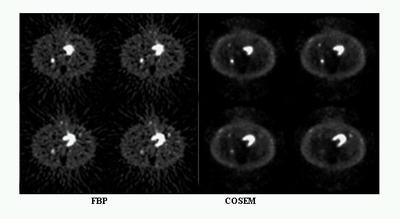 Fig. 3.8. : Comparison between images of the Lung and Heart phantom with 4 inserts (Duke Hospital, USA) reconstructed by standard filtered backprojection (left) and images reconstructed using COSEM optimised iterative reconstruction (right)
The smallest observable sphere has a radius of 8 mm (Courtesy of Dr R. Levkovitz, Technion).
3.5.2 OSEM with inter-update filtering
An enhanced version of OSEM called Inter-Update Metz Filtered OSEM (IUMF-OSEM), which uses an iterative filtering technique for enhancing image quality was developed by Jacobson et al (1999). In this technique, a Metz filter is applied to image estimates at certain intervals. This filter is known to carry out restorative image enhancement on the image estimates, and the proposed algorithm incorporates it in OSEM's updating mechanism.
A software implementation of IUMF-OSEM was performed using the previously described object-oriented library for 3D PET reconstruction (Labbé et al 1999b). The algorithm combines the forward and back projection operators with an appropriate choice of ordered sets to fully use all symmetry properties for fast computation.
The performance of IUMF-OSEM Vs standard OSEM and post-filtered OSEM reconstructions was tested on phantom and clinical studies. The phantom scans were acquired on the GE-Advance PET scanner. Data sets were pre-corrected for attenuation, detector efficiency, scatter, and random coincidences. Iterative filtering operations were applied at intervals of full iterations. Fig. 3.9 shows sample images of the Jaszczak phantom reconstructed with 14 subsets and 5 iterations (70 sub-iterations).
Quantitative evaluations of the algorithm on phantom data showed that inter-update Metz filtering, with appropriately chosen filter parameters yields superior signal-to-noise ratio and contrast recovery compared to plain OSEM. Moreover, contrast enhancement was found to be higher, and noise control only slightly poorer than that obtained by post-filtered OSEM. The contrast enhancing capability of IUMF-OSEM was also demonstrated on reconstructions of the whole body phantom and on clinical studies.
 Fig. 3.9. : Illustration of the Jaszczak phantom with rods insert (left) and a sample IUMF-OSEM reconstruction (slice 16) after 70 iterations with Metz filter power 1, radial FWHM is 5 mm and axial FWHM is 8 mm (right)
(Jacobson et al 1999)
Fig. 3.9. : Illustration of the Jaszczak phantom with rods insert (left) and a sample IUMF-OSEM reconstruction (slice 16) after 70 iterations with Metz filter power 1, radial FWHM is 5 mm and axial FWHM is 8 mm (right)
(Jacobson et al 1999)
3.5.3 The mirror descent algorithm
A new numerical method called Ordered Subsets Mirror Descent (OSMD) for solving a non-smooth convex optimisation problem over a compact feasible set was recently introduced and applied to the problem of image reconstruction in 3D PET (Ben-Tal et al 1999). This is an accelerated version of the Mirror Descent (MD) method developed by Nemirovski and Yudin (1978). The MD method can be regarded as a non-Euclidean version of the classical subgradient method, but has a significant theoretical advantage since its rate of convergence is independent (or nearly so) of the dimension of the problem. This feature makes it an attractive choice for large-scale problems like volumetric reconstruction of PET data.
The OSMD algorithm has been adapted to the PET reconstruction by reformulating the optimisation problem. This leads to an objective function and a constraining set with desirable properties. A proof of convergence of the OSMD method for the unconstrained case and for a constrained compact convex domain together with more details about the algorithm are described elsewhere (Ben-Tal et al 1999). A principal advantage of OSMD is that convergence to the maximum likelihood estimate is guaranteed for any choice of subsets and for any projection data. OSEM on the other hand may cycle among sub-optimal solutions if the data are noisy and/or the subsets don't satisfy certain balancing conditions described in Hudson and Larkin (1994). It is worth to point out that the preliminary results presented here come from a prototype implementation. A more comprehensive evaluation is in preparation by the authors of this algorithm. Fig. 3.10 shows slices of a Monte Carlo simulated Jaszczak phantom with rods insert for the PRT-1 tomograph reconstructed with both OSMD (left) and standard OSEM (right). The OSMD reconstruction exhibits high resolution even for the block with the smallest diameters.
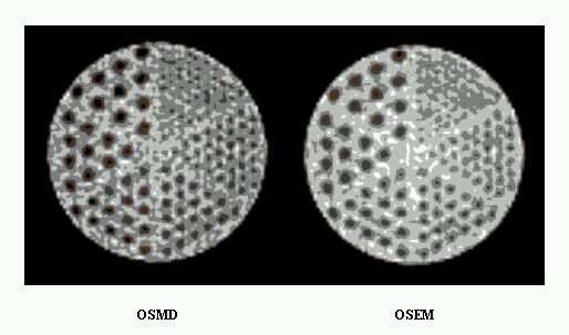 Fig. 3.10. : One slice of a simulated Jaszczak phantom with rods insert reconstructed with OSMD (left) and standard OSEM (right) after 5 iterations with 6 subsets
(Ben-Tal et al 1999)
Fig. 3.10. : One slice of a simulated Jaszczak phantom with rods insert reconstructed with OSMD (left) and standard OSEM (right) after 5 iterations with 6 subsets
(Ben-Tal et al 1999)
3.5.4 Inverse Monte Carlo-based reconstruction
The concept of inverse Monte Carlo (IMC) was introduced in 1981 in an attempt to describe a numerical method for solving a class of inverse problems (Dunn 1981). The IMC method converts the inverse problem, through a non-iterative simulation technique, into a system of algebraic equations that can be solved by standard analytical or numerical techniques. The principal merits of IMC are that, like direct Monte Carlo, the method can be applied to complex and multivariable problems, and variance reduction procedures can be applied. The non-iterative IMC is strongly related to the variance reduction technique in direct simulation called importance sampling where the sampling process is altered by using random numbers from a modified distribution.
Application of the Monte Carlo method for solving the inverse problem in emission computed tomography has been previously reported by other groups (Floyd et al 1986). As proposed, the method realises tomographic reconstruction for SPECT with simultaneous compensation for attenuation, scatter, and distance-dependent collimator resolution. A detection probability matrix was created by Monte Carlo solution to the photon transport equation for a simulated SPECT acquisition from a unit source activity in each source voxel. The measured projection vector equals the product of this detection probability matrix with the unknown source distribution vector. The resulting large, non-sparse system of equations was solved for the source distribution using an iterative ML-EM estimator. It is worth to note that although the technique was developed for SPECT, it is also valid for other imaging techniques like PET and transmission CT.
A strategy for developing a 3D reconstruction algorithm for PET based on IMC taking advantage of the fact that Monte Carlo methods provide a natural framework for incorporation of detector response function, the effects of attenuation, scatter and other sources of systematic errors in the transition matrix is presented here and further discussed in future developments section (chapter 8). Our proposed application of IMC is in the context of the 3D ML-EM reconstruction algorithm (see section 3.2.2). For each iteration, the update to the source distribution is done by comparing the forward projected data of the current image estimate to the measured projections. The IMC procedure replaces the explicit forward projection step given by Eq. (3.12) in the ML-EM algorithm as  by Monte Carlo generated events according to a hypothesised source distribution and attenuation map. A uniform image could be used as the initial source estimate for the first iteration. In the following iterations, voxel values are updated by the ratio of the backprojection of the measured data to the Monte Carlo generated data at that voxel. The total number of detected events is scaled to match the original measured data sets.
A preliminary version of the IMC algorithm was implemented using the 3D reconstruction library (Labbé et al 1999b). Our approach may be distinguished from the method of Floyd et al (1986) and has been discussed as a potential application of our Monte Carlo simulator (Zaidi et al 1998), although other groups reported some related work in progress in the context of the image space reconstruction algorithm (Kudrolli et al 1999). One of the limitations of their work is the rather crude system model used which contains only the basic detector geometry. That is, the system response matrix  is approximated by the length of intersection of the ith LOR with the jth voxel. A major advantage of our approach is that is avoids the explicit calculation and storage of the system response matrix since Monte Carlo simulation of a given source/scattering/detector system implicitly contains all the information contained in the detection probability matrix. The probability matrix is usually much too large to store in memory and has to be either stored on disk or calculated on the fly. Several groups have used symmetries and sparsness of this matrix to be able to store it in memory (Qi et al 1998).
Obviously, IMC is a reconstruction algorithm which is based on a more realistic model of the PET acquisition process. The most dramatic improvements using IMC are expected to be apparent for low statistics studies. This is significant since clinical PET studies are usually count limited. This improvement in image noise is expected to be to due to several characteristic features of IMC: the incorporation into the EM algorithm of the knowledge that the photon counting process follows a Poisson distribution, the simultaneous solution approach, and the detailed modelling provided by the Monte Carlo method reduces the data inconsistency. The most effective clinical application of IMC could be envisaged in studies where the signal to noise ratio is too low for conventional FBP or common iterative reconstruction techniques. Specific applications include fast dynamic studies and low statistics multi-bed oncologic studies. The most obvious disadvantage of the IMC algorithm is the increased computational effort required to perform the reconstructions. However, parallel implementation may help to overcome this drawback.
3.5.5 Parallelisation and scalability
As stated previously, the major goal of the PARAPET project is to create parallel versions of both analytic and iterative algorithms to run on distributed memory multiprocessor parallel platforms. The partners in the project use Parsytec CC series of systems (Fig. 3.11), however, the main goal is to create parallel software tools that achieve:
-
speed-up on the basis of elapsed wall-clock time;
-
scale-up in terms of the size of data sets obtained on different scanners;
-
portability and platform independence, allowing to run the software on clusters of high-end PCs and workstations and other distributed memory multiprocessor hardware architectures.
The parallelisation library developed by our partners (sadki et al 1999) provides the programmer with a common interface for creating parallel applications for different hardware and software platforms. Both PVM (Geist et al 1994) and EPX (EPX 1996) message-passing libraries are supported now, and it is planned that MPI will be supported in the near future. The library consists of a set of C++ classes and functions that define a common parallel programming interface independent of a particular message-passing library. Therefore, the application is definitely isolated from the used low-level library. Moreover, the implemented message-passing code can be used as it is when ported to a different hardware platform (as far as the platform is supported by the library).
 Fig. 3.11. : Photograph of the 8-node Parsytec CC system installed at Geneva University Hospital
Parallel implementation of the reconstruction algorithms uses this portable, object-oriented message passing library and a coarse-grain parallelisation approach based on partitioning the projection space. By considering similarity with respect to data distribution and communication patterns, four groups of parallel reconstruction algorithms were identified :
-
3DRP, FORE, ...etc.
-
OSEM, OSEM/MAP, OSMD, BI-SMART;
-
pure ART and modifications of ART based on splitting the image volume;
-
B-ART.
Detailed analysis of data flow allowed to identify and parallelise a common kernel. For example, 3DRP, which is an analytic algorithm, shares the same strategy with OSEM, but is classified in a separate group due to its differences from the OSEM-like schemes. With current and future developments, more groups of algorithms can be identified and corresponding parallel kernels implemented. For the present implementation, a master-slave architecture was adopted. The processing time depends on data sizes and hence on the segment number (ring difference) being processed. This results in a problem of even distribution of the workload which was handled by implementing on-the-fly workload distribution scheme. In this approach, the working nodes are assigned jobs as soon as they get free, instead of using a predefined partitioning scheme. Since the size of projection data decreases with increasing ring difference, processing ring differences in ascending order seems a reasonable solution. This leads to better load balancing and allows to reduce the granularity of required processing towards the end of a sub-iteration. The achieved speed-up will of course be influenced by the different sizes of projections. The strategy adopted for data decomposition consists in partitioning the projection space across the processors (Sadki et al 1999). For instance, in the case of OSEM, this approach assigns groups of symmetry-related viewgrams to different processors, and allows several iterations of the inner loop to be executed in parallel. Data consolidation involves summing the partial computations of the update factors calculated on different processors.
Performance evaluation was carried out on the Parsytec CC system consisting of 12 nodes (see chapter 6 for a detailed description of the system). Reconstructions were carried out for data sets of both PRT-1 and GE-Advance tomographs. Scalability issues were investigated by varying the number of nodes from 3 to 12. The efficiency of the parallelisation approach for different numbers of nodes was assessed by comparing parallel timing results with those obtained by running the code in serial mode. In the present implementation, the master node is used only for data distribution and load balancing. Efficiency is therefore defined as  , where N is the total number of nodes.
Timing results and parallelisation efficiencies together with estimated timings for an 'ideal' case of linear speed-up defined as  for two different scanners are presented in Fig. 3.12. As can be seen on the illustrated charts, the parallel implementation provides a reasonable speed-up and leads to reduced reconstruction times. In particular, the implementation on 12 nodes yielded a speed-up relative to serial mode of about 7 out of a possible 11. Comparison of efficiency charts for PRT-1 and GE-Advance scanners suggests that the implementation scales well with respect to problem size. The parallelisation of the algorithms constitutes a significant step toward achieving clinically acceptable reconstruction times.
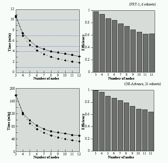 Fig. 3.12. : Execution time per iteration (left) and efficiency (right) of parallel implementation of OSEM algorithm on the Parsytec CC system for both PRT-1 (top) and the GE-Advance (bottom) scanners
Both actual execution time (circles) and estimated timings for an 'ideal' case of linear speed-up (diamonds) are shown (Sadki et al 1999).
4. Monte Carlo modelling in positron emission tomography
Monte Carlo techniques have become popular in different areas of medical physics with advantage of powerful computing systems. In particular, they have been extensively applied to simulate processes involving random behaviour and to quantify physical parameters that are difficult or even impossible to calculate by experimental measurements. Recent nuclear medical imaging innovations such as SPECT, PET, and MET are ideal for Monte Carlo modelling techniques because of the stochastic nature of radiation emission, transport and detection processes. Factors which have contributed to the wider use include improved models of radiation transport processes, the practicality of application with the development of acceleration schemes and the improved speed of computers. This chapter presents derivation and methodological basis for this approach and summarises their areas of application in PET imaging. An overview of existing simulation programs is provided and illustrated with examples of some useful features of such sophisticated tools in connection with common computing facilities and more powerful multiple-processor parallel processing systems.
Recent developments in nuclear medicine instrumentation and multiple-processor parallel processing systems have created new opportunities for Monte Carlo simulation in nuclear medicine imaging. One of the aims of the medical physicist involved in nuclear medical imaging research is to optimise the design of imaging systems and to improve the quality and quantitative accuracy of reconstructed images. Several factors affect the image quality and the accuracy of the data obtained from a nuclear medicine scan. These include the physical properties of the detectors, collimator and gantry design, attenuation and scatter compensation, and reconstruction algorithms (Zaidi 1996b). Integrating improvements in these with current tracers and sensitive and specific tracers under development will provide major advantages to the general nuclear medicine clinician and research investigator (Fig. 3.1). Mathematical modelling is necessary for the assessment of various parameters in nuclear medical imaging systems since no analytical solution is possible when solving the transport equation describing the interaction of photons with non-uniformly attenuating body structures and complex detector geometries.
The main purpose of this chapter is to present a framework for applying Monte Carlo simulations for a wide range of problems in positron emission tomography. Emphasis is given to applications where photon and/or electron transport in matter is simulated. Some computational aspects of the Monte Carlo method, mainly related to random numbers, sampling and variance reduction are discussed and followed by the presentation of potential applications of Monte Carlo techniques in different areas of PET imaging such as detector modelling and systems design, image reconstruction and scatter correction techniques, internal dosimetry and pharmacokinetic modelling. Widely used Monte Carlo codes in connection with computing facilities, vectorized and parallel implementations are described.
 Fig. 4.1. : Scientific and technical strategy for recording accurate functional images
(adapted from an illustration by Prof. Terry Jones, MRC, UK)
Fig. 4.1. : Scientific and technical strategy for recording accurate functional images
(adapted from an illustration by Prof. Terry Jones, MRC, UK)
In bold, the parts where Monte Carlo simulation plays an important role.
4.1 The Monte Carlo method
The Monte Carlo method is widely used for solving problems involving statistical processes and is very useful in medical physics due to the stochastic nature of radiation emission, transport and detection processes. The method is very useful for complex problems that cannot be modelled by computer codes using deterministic methods or when experimental measurements may be impractical. The Monte Carlo method was named by Von Neumann (McCracken 1955) because of the similarity of statistical simulation to games of chance, and because the city in the Monaco principality was a centre for gambling and similar pursuits. Von Neumann, Ulam, and Fermi applied the method towards neutron diffusion problems in the Manhattan Project at Los Alamos during World War II. But, even at an early stage of these investigations, von Neumann and Ulam refined this particular 'Russian roulette' and 'splitting' methods. However, the systematic development of these ideas had to await the work of Kahn and Harris in 1948 (Kahn 1956). During the same year, Fermi, Metropolis, and Ulam obtained Monte Carlo estimates for the eigenvalues of Schrodinger equation. Uses of Monte Carlo methods have been many and varied since that time. The applications of the Monte Carlo method in medical physics were few before the review paper by Raeside (1976). Since that time, there has been an increasing number of applications of Monte Carlo techniques to problems in this field thanks to the several books (Jenkins 1988, Morin 1988, Nahum 1989, Lux 1991, Ljungberg et al 1998) and comprehensive review papers (Raeside 1976, Turner et al 1985, Andreo 1991, Zaidi 1999a) describing the principles of the Monte Carlo method and its applications in medical physics.
Numerical methods that are known as Monte Carlo methods can be loosely described as statistical simulation methods, where statistical simulation is defined in quite general terms to be any method that utilises sequences of random numbers to perform the simulation. A detailed description of the general principles of the Monte Carlo method is given in a number of publications (Raeside 1976, Turner et al 1985) and will not be repeated here. The major components of a Monte Carlo method are briefly described below. These components comprise the foundation of most Monte Carlo applications. The following sections will explore them in more detail. An understanding of these major components will provide a sound foundation for the developer to construct his own Monte Carlo method. The primary components of a Monte Carlo simulation method include the following:
-
Probability density functions (pdf's): the physical system must be described by a set of pdf's.
-
Random number generator: a source of random numbers uniformly distributed on the unit interval must be available.
-
Sampling rule: a prescription for sampling from the specified pdf's.
-
Scoring: the outcomes must be accumulated into overall tallies or scores for the quantities of interest.
-
Error estimation: an estimate of the statistical error (variance) as a function of the number of trials and other quantities must be determined.
-
Variance reduction techniques: methods for reducing the variance in the estimated solution to reduce the computational time for Monte Carlo simulation.
-
Parallelisation and vectorisation algorithms to allow Monte Carlo methods to be implemented efficiently on advanced computer architectures.
4.2 Computational methods
4.2.1 Random numbers generation
Computational studies requiring the generation of random numbers are becoming increasingly common. All random number generators (RNG) are based upon specific mathematical algorithms, which are repeatable. As such, the numbers are just pseudo-random. Here, for simplicity, we shall term them just 'random' numbers. Formally, random is defined as exhibiting 'true' randomness, such as the time between 'tics' from a Geiger counter exposed to a radioactive element. Pseudo-random is defined as having the appearance of randomness, but nevertheless exhibiting a specific, repeatable pattern. Quasi-random is defined as filling the solution space sequentially (in fact, these sequences are not at all random, they are just comprehensive at a preset level of granularity). Monte Carlo methods make extensive use of random numbers to control the decision making when a physical event has a number of possible results. The RNG is always one of the most crucial subroutines in any Monte Carlo-based simulation code. A large number of generators are readily available (Marsaglia and Zaman 1994), and many of these are suitable for implementation on any computer system since today there is no significant distinction in floating point processing capabilities between a modern desktop and a mainframe computer. A typical simulation uses from 107 to 1012 random numbers, and subtle correlations between these numbers could lead to significant errors (Ferrenberg et al 1992). The largest uncertainties are typically due more to approximations arising in the formulation of the model than those caused by lack of randomness in the RNG. Mathematically speaking, the sequence of random numbers used to effect a Monte Carlo model should possess the following properties (Vattulainen et al 1995):
-
Uncorrelated sequences: the sequences of random numbers should be serially uncorrelated. Most especially, n-tuples of random numbers should be independent of one another.
-
Long period: ideally, the generator should not repeat; practically, the repetition should occur only after the generation of a very large set of random numbers.
-
Uniformity: the sequence of random numbers should be uniform, and unbiased. That is, suppose we define n-tuples
 and divide the n-dimensional unit hypercube into many equal sub-volumes. A sequence is uniform if in the limit of an infinite sequence, all the sub-volumes have an equal number of occurrences of random n-tuples.
-
Reproducibility: when debugging programs, it is necessary to repeat the calculations to find out how the errors occurred. The feature of reproducibility is also helpful while porting the program to a different machine
-
Speed: it is of course desirable to generate the random numbers fast.
-
Parallelisation: the generator used on vector machines should be vectorisable, with low overhead. On massively parallel architectures, the processors should not have to communicate among themselves, except perhaps during initialisation.
Although powerful RNGs have been suggested including shift register, inversive congruentional, combinatorial and 'intelligent' methods such as those implemented in the MCNP code (Booth 1988), the most commonly used generator is the linear congruential RNG (LCRNG) (Lehmer 1949). Recently, Monte Carlo researchers have become aware of the advantages of lagged Fibonacci series (LFRNG). With extremely long periods, they are generally faster than LCRNG and have excellent statistical properties (Marsaglia and Zaman 1993). Those generators are briefly described below.
4.2.1.1 Linear Congruential Generators
The LCRNG has the form (Lehmer 1949) :
 |
(4.1) |
where m is the modulus, a the multiplier, and c the additive constant or addend. The size of the modulus constrains the period, and is usually chosen to be either prime or a power of 2 (Knuth 1981). An important subset of LCRNG is obtained by setting c=0 in Eq. (4.1), which defines the multiplicative linear congruential RNG (MLCRNG). This generator (with m a power of 2 and c=0) is the de facto standard included with FORTRAN and C compilers (Press 1992). One of the biggest disadvantages to using a power of 2 modulus is that the least significant bits of the integers produced by these LCRNGs have extremely short periods. For example,  will have a period of 2j (Knuth 1981). In particular, this means the least-significant bit of the LCRNG will alternate between 0 and 1. Some cautions to the programmer are in order: (i) the bits of un should not be partitioned to make several random numbers since the higher order bits are much more random than the lower order bits; (ii) the power of 2 modulus in batches of powers of 2 should be avoided; (iii) RNGs with large modulus are preferable to ones with small modulus. Not only is the period longer, but the correlations are lower. In particular, one should not use 32 bit modulus for applications requiring a high resolution in the random numbers. In spite of this known defect of power of 2 LCRNGs, 48 bit multipliers (and higher) have passed many very stringent randomness tests.
The initial seed should be set to a constant initial value, such as a large prime number (it should be odd, as this will satisfy period conditions for any modulus). Otherwise, the initial seed should be set to a 'random' odd value. Anderson (1990) recommends setting the initial seed to the following integer :
 |
(4.2) |
where the variables on the right-hand side are the integer values of the date and time. Note that the year is 2 digits long, i.e. the domain of iyr is [0-99]. However, it may be preferable to introduce the maximum variation in the seed into the least significant bits by using the second of this century, rather than the most significant bits. The following equation is preferable :
 |
(4.3) |
Generally LCRNGs are best parallelised by parametrizing the iteration process, either through the multiplier or the additive constant. Based on the modulus, different parametrizations have been tried (Anderson 1990).
4.2.1.2 Lagged-Fibonacci Generators
The lagged-Fibonacci series RNG (LFRNG) have the following general form (Marsaglia and Zaman 1994) :
 , l > ; k , l > ; k |
(4.4) |
where  may be one of the following binary arithmetic operators +, -, *; l and k are the lags, and m is a power of 2 (m=2p). In recent years the additive lagged Fibonacci RNG (ALFRNG) has become a popular generator for serial as well as scalable parallel machines (Mascagni et al 1995) because it is easy to implement, it is cheap to compute and it does well on standard statistical tests, especially when the lag k is sufficiently high (such as k = 1279). The maximal period of the ALFRNG is
  and has
  different full-period cycles (Brent 1994). Another advantage of the ALFRNG is that one can implement these generators directly in floating-point to avoid the conversion from integer to floating-point that accompanies the use of other generators. However, some care should be taken in the implementation to avoid floating point round-off errors.
Instead the ALFRNG can be parameterized through its initial values because of the tremendous number of different cycles. Different streams are produced by assigning each stream a different cycle. An elegant seeding algorithm that accomplishes this is described by Mascagni et al (1995). An interesting cousin of the ALFRNG is the multiplicative lagged-Fibonacci RNG (MLFRNG). While this generator has a maximal-period of  , which is a quarter the length of the corresponding ALFRNG, it has empirical properties considered to be superior to ALFRNGs (Marsaglia and Zaman 1994). Of interest for parallel computing is that a parametrization analogous to that of the ALFRNG exists for the MLFRNG.
4.2.2 The source and positron emission
In most Monte Carlo computer codes, the positron histories and thus positron range are neglected during simulations with the assumption that the positron emission point is coincident with the annihilation point. The annihilation point in the source region and the flight direction for the first of the two annihilation 511 keV photons are randomly generated. The second annihilation photon is generated in the same emission position, but with anti-parallel flight direction with respect to the first one. Both the positron range and the non-collinearity effects are accounted for by analytic models and included with the other physical phenomena affecting spatial resolution.
4.2.3 Modelling photon transport
For radiation transport problems, the computational model includes geometry and material specifications. Every computer code contains a database of experimentally obtained quantities, known as cross sections, that determine the probability of a particle interacting with the medium through which it is transported. Every cross section is peculiar to the type and energy of the incident particle and to the kind of interaction it undergoes. These partial cross sections are summed to form the total cross section; the ratio of the partial cross section to the total cross section gives the probability of this particular interaction occurring. Cross section data for the interaction types of interest must be supplied for each material present. The model also consists of algorithms used to compute the result of interactions (changes in particle energy, direction, etc.) based on the physical principles that describe the interaction of radiation with matter and the cross section data provided. Therefore, it is extremely important to use an accurate transport model as the Monte Carlo result is only as valid as the data supplied.
When a photon (having an energy below 1 MeV) passes through matter, any of the three interaction processes (photoelectric, incoherent scattering, coherent scattering) may occur. The probability of a photon of a given energy E undergoing absorption or scattering when traversing a layer of material Z can be expressed quantitatively in terms of a linear attenuation coefficient  (cm-1) which is dependent on the material's density, r (g.cm-3).
In the case of photoelectric absorption, the total photon energy is transferred to an atomic electron and the random walk is terminated. In an incoherent photon interaction, a fraction of the photon energy is transferred to the atomic electron. The direction of the scattered photon is changed to conserve the total momentum of the interaction. The Klein-Nishina expression for the differential cross section per electron for an incoherent interaction is used to sample the energy and the polar angle of the incoherently scattered photon (Klein and Nishina 1928). The coherent scattering only results in a change in the direction of the photon since the momentum change is transferred to the whole atom. The kinetic energy loss of the photon is negligible. Coherent scattering of a photon could be generated using the random number composition and rejection technique (Kahn 1956) to sample the momentum of the scattered photon and the scattering angle according to the form factor distribution. A simplified flow chart of photon transport for the energies of interest in nuclear medicine imaging is given in Fig. 4.2.
 Fig. 4.2. : A flow diagram showing the main steps followed when simulating a photon transport history
It is common to neglect coherent scattering in PET Monte Carlo simulation of photon transport because of its low contribution to the total cross section at 511 keV. In the following examples, the relative importance of the various processes involved in the energy range of interest (below 1 MeV) are considered for some compounds and mixtures used in nuclear medicine to justify some of the approximations made in Monte Carlo codes. Fig. 4.3 illustrates the relative strengths of the photon interactions versus energy for water, cortical bone, sodium iodide (NaI(Tl)) and bismuth germanate (BGO), respectively. For water, a moderately low-Z material, we note two distinct regions of single interaction dominance: photoelectric below and incoherent above 20 keV. The almost order of magnitude depression of the coherent contribution is some justification for the approximations discussed. The coherent contribution to the total cross section is less than 1% for energies above 250 keV. However, this contribution is in the order of 7% for high-Z materials like BGO. Therefore, efforts should be made to treat the coherent scattering process adequately for detector materials.


 Fig. 4.3. : Components of photon cross sections for different tissues (H2O and cortical bone) and detector materials (NaI(Tl) and BGO) of interest in PET imaging illustrating the relative contribution of each process
Calculation of the distances between interactions in a medium are performed by sampling from the exponential attenuation distribution (Eq. 4.8 below). Different techniques have been proposed to improve the computation speed when sampling from the probability distributions. They are described in more detail in the following sections.
In principle, electron transport should be included when simulating the complete electromagnetic cascade (microscopic techniques). However, the large number of interactions that may occur during electron slowing down makes it unrealistic to simulate all the physical interactions (macroscopic techniques). Secondary electrons are generally assumed to deposit all their energy at the point of interaction because of the low energies involved in nuclear medicine and therefore the short ranges of the electrons generated and their negligible Bremsstrahlung production. Therefore, electron transport has not received particular attention in nuclear imaging applications of the Monte Carlo method. However, a number of investigators considered this effect mainly for dosimetry calculations (Furhang et al 1997).
4.2.4 Analogue sampling
Analogue Monte Carlo attempts to simulate the full statistic development of the electromagnetic cascade. If we assume that a large number of particle histories, N, are included in a batch, the individual batch estimates can be considered as drawn from a normal distribution. For a given calculation, the estimated uncertainty is proportional to the inverse of the square root of the number of histories simulated. The efficiency  of a Monte Carlo calculation can therefore be defined as (Bielajew and Rogers 1989):
 |
(4.5) |
where T is the calculation time required to obtain a variance estimate  . For large N,
  should be constant as long as the calculation technique remains the same.
As discussed earlier, the imaging system can be described in terms of pdf's. These pdf's, supplemented by additional computations, describe the evolution of the overall system, whether in space, energy, time, or even some higher dimensional phase space. The goal of the Monte Carlo method is to simulate the imaging system by random sampling from these pdf's and by performing the necessary supplementary computations needed to describe the system evolution. In essence, the physics and mathematics are replaced by random sampling of possible states from pdf's that describe the system. Thus, it is frequently necessary to sample some physical event, the probability of which is described by a known pdf. Examples include the distance to the next interaction and the energy of a scattered photon. Let x be the physical quantity to be selected and f(x) the pdf. Among the properties of the pdf is that it is integrable and non-negative. Assume that the domain of f(x) is the interval [xmin, xmax] and that it is normalised to unit area. The cumulative distribution function F(x) of the frequency function f(x) gives the probability that the random variable t is less or equal to x. It is defined as:
 , , |
(4.6) |
A stochastic variable can be sampled by the use of uniformly distributed random numbers R in the range [0-1] using one of the techniques described below.
4.2.4.1 Direct method
This method can be used if the inverse of the cumulative distribution function F-1(x) is easily obtainable. Since F(x) is uniformly distributed in [0-1], the sampled value of x could be obtained by substituting F(x) in Eq. (4.6) by a uniform random number R, that is  . A practical example of using this technique is the calculation of the distance to the next interaction vertex. The inversion is not always possible, but in many important cases the inverse is readily obtained.
4.2.4.2 Rejection method
Another method of performing this when it is too complicated to obtain the inverse of the distribution function is to use the rejection technique (Kahn 1956) which follows the following steps :
-
define a normalised function
 , where fmax(x) is the maximum value of f(x),
-
sample two uniformly distributed random numbers R1 and R2,
-
calculate x using the equation
 ,
,
-
if R2 is less than or equal to f'(x) then x is accepted as a sampled value, otherwise a new value of x is sampled.
Over a large number of samples, this technique will yield a set of values of x within the required distribution. It does, however, require two random numbers per trial and many trials may be required depending on the area under of the curve of f(x). A typical example of using this technique is the sampling of the photon energy and scattering angle resulting from incoherent scattering.
4.2.5 Non-analogue sampling "Variance reduction techniques"
A direct Monte Carlo simulation using true probability functions may require an unacceptable long time to produce statistically relevant results. Photons emission is isotropic, so directional parameters may be sampled uniformly within their individual ranges. Nuclear imaging systems have a low geometrical efficiency because of the small solid angle defined by the collimator and/or the small axial aperture. Therefore, the calculation would be very ineffective in terms of required computing time (Haynor et al 1990). It is thus desirable to bias the sampling (non-analogue sampling) by introducing different types of importance sampling and other variance reduction techniques to improve the computational efficiency of the Monte Carlo method (Zubal and Harell 1992). The results obtained by non-analogue simulation are, however, biased by the variance reduction technique and a correction for this is required. A particle history weight, W, is introduced, which describes the probability of the particle following the current path. This weight is calculated for each particle history, and used in the calculation of the results. If an event occurs, the weight W is added to the counter rather than incrementing the counter by one unit. Bielajew and Rogers (1989) divided variance reduction techniques in three categories: those that concern photon transport only, those that concern electron transport only, and other more general methods. The most useful techniques in photon transport are described below. It is worth to note that concerning the Poisson nature of the activity distributions in PET, these variance reduction approximations may result in statistically relevant deviations from an otherwise unbiased simulation result since Monte Carlo simulated projection data are (as a result of variance reduction) not count but probability data.
4.2.5.1 Interaction forcing
In an analogue Monte Carlo simulation, photons are tracked through the object until they either escape the object, are absorbed, or their energy drops below a selected threshold. The probability function for a photon interaction is given by:
 |
(4.8) |
The probability that a photon will travel a distance d or less is given by:
 |
(4.9) |
To sample the pathlength, a uniform random number R is substituted for p(d) and the problem is solved for d:
 |
(4.10) |
Since the maximum distance, dmax, the photon travels before interaction is infinite and the number of mean free paths across the geometry in any practical situation is finite, there is a large probability that photons leave the geometry of interest without interacting. To increase the statistical accuracy in the imparted energy calculation, we force the photons to interact by assigning dmax a finite distance, e.g. the thickness of the detector being simulated. A true distributed photon pathlength d within dmax can be sampled from the equation:
 |
(4.11) |
The photon's weight must be multiplied by the interaction probability:
 |
(4.12) |
In emission computed tomography, the photon is allowed to interact through coherent or incoherent interactions only within the phantom since photo-absorption does not contribute to energy imparted in the crystal. The weight is then multiplied by the probability for the photon being scattered:
 |
(4.13) |
where  and
and  are the cross section data for incoherent and coherent scattering, respectively, and
  is the total linear attenuation coefficient.
4.2.5.2 Stratification
Stratification refers to the process of determining the frequencies with which the various regions of state space are used to start a particle (Haynor et al 1991). The solid angle of acceptance of the detector array,  is small due to collimation and to the size of the detector array itself. This results in significant computational inefficiencies with analogue Monte Carlo simulation, because only a few percent of the photons generated and tracked will actually be detected. The goal of stratification is to simulate only photons that are emitted in directions within the solid angle which can be calculated from the maximum acceptance angle,
  , which in turn can be estimated from the dimensions of the phantom and the detection system. The solid angle doesn't change in magnitude when simulating source locations off-centre. The photon escaping from the phantom is either primary or scattered. If the photon happens to be a primary photon, its direction within the solid angle could be sampled from
 |
(4.14) |
In this case, the weight is multiplied by the probability of escape without interaction in the solid angle 
 . . |
(4.15) |
4.2.5.3 Exponential transform, Russian roulette and particle splitting
The exponential transform is a variance reduction technique used to bias the sampling procedure to give more interactions in the regions of interest and thus improve the efficiency of the calculation for those regions. To implement this method, the distance to the next interaction in number of mean free paths,  , should be sampled from (Bielajew and Rogers 1989):
 |
(4.16) |
where C is a parameter that adjusts the magnitude of the scaling and  the angle of the photon with respect to the direction of interest. The new weighting factor is given by
 |
(4.17) |
Note that the new weighting factor is dependent on  . If
. If  , the particle pathlength is stretched in the forward direction, which is used for shielding problems. For
  , the average distance to the next interaction is shortened in the forward direction, which is used for surface problems. For
  , we recover the unbiased sampling. The optimal choice of this parameter is dependent on the problem to be solved. The general guideline is to avoid to use large weighting factors because they may increase the variance.
Russian roulette and splitting are often used together with the exponential transform, although they are still effective when used independently. In Russian roulette, a random number is selected and compared to a threshold,  . If the random number turns out to be smaller than
  , the particle is allowed to survive but the weight should be updated accordingly:
  . In particle splitting, a particle coming from a region of interest can be divided into N particles, each having a new weighting:
  .
.
4.2.5.4 Correlated sampling
The correlated sampling technique can be used in transport of both photons and electrons. It is especially effective for calculating ratios or differences of two quantities which are nearly equal. The basic idea is that the simulations of the geometries of interest are kept as closely correlated as possible so that most of the statistical fluctuations will cancel in the ratios and differences. The real difference between the two geometries will be better reflected in the ratios and the differences obtained. The calculational uncertainties in the ratios and the differences obtained with correlated sampling are in general smaller than those obtained from uncorrelated simulations.
There are several ways of doing correlated sampling in radiation transport. In coupled photon-electron transport, a simple method has been used in which random number seeds of the particle histories, for which a primary particle or any of the secondaries has deposited energy in the region of interest for one geometry, is stored and used for the simulations of the alternative geometry (Bielajew and Rogers, 1989). A new correlated sampling method for the transport of electrons and photons has been developed in which a main particle history is split up whenever a particle meets the boundary of the region where the medium differs between the two or more cases (Ma and Nahum 1993). This particle is then followed separately for each case until it and all its descendants terminate.
4.2.5.5 Use of geometry symmetry
The use of some of the inherent symmetry of the geometry may realise considerable increase in efficiency. If both the source and target configurations contain cylindrical planar or spherical-conical simulation geometries, the use of symmetries is more obvious. Other uses of symmetry are less obvious but the saving in computing time is worth the extra care and coding.
4.3 Applications of the Monte Carlo method in positron emission tomography
There has been an enormous increase and interest in the use of Monte Carlo techniques in all aspects of nuclear imaging, including planar imaging (Webb et al 1992), SPECT (Ljungberg and Strand 1989, DeVries et al 1990), PET (Keller and Lupton 1983, Dahlbom et al 1989, Zaidi et al 1999a), and MET (Dahlbom et al 1998). However, due to computer limitations, the method has not yet fully lived up to its potential. With the advent of high-speed supercomputers, the field has received increased attention, particularly with parallel algorithms which have much higher execution rates.
Fig. 4.4 illustrates the idea of Monte Carlo or statistical simulation as applied to an imaging system. Assuming that the behaviour of the imaging system can be described by probability density functions (pdf's), then the Monte Carlo simulation can proceed by sampling from these pdf's, which necessitates a fast and effective way to generate random numbers uniformly distributed on the interval [0,1]. Photon emissions are generated within the phantom and are transported by sampling from pdf's through the scattering medium and detection system until they are absorbed or escape the volume of interest without hitting the crystal. The outcomes of these random samplings, or trials, must be accumulated or tallied in an appropriate manner to produce the desired result, but the essential characteristic of Monte Carlo is the use of random sampling techniques to arrive at a solution of the physical problem.
 Fig. 4.4. : Principles of Monte Carlo simulation of a nuclear medical imaging system
4.3.1 Detector modelling
The critical component of emission tomography is the scintillation detector. Monte Carlo simulation of detector responses and efficiencies is one of the areas which has received considerable attention (Andreo 1991, Zaidi 1999a). An early contribution to the field providing a detailed description of the techniques used was due to Zerby (1963). Many detector modelling applications were developed in the PET field including the pioneering work of Derenzo (1981) who simulated arrays of detectors of different materials and sizes to study the effect of the inter-crystal septa and later on to optimise the optical coupling between BGO crystals and PMT's (Derenzo and Riles 1982) by taking into account the reflection and scattering along the detection system. The search for an appropriate detector for this imaging modality was conducted in a comparative study of several crystals including BGO, CsF and NaI(Tl) (Bottigli et al 1985), BaF2 used in time-of-flight PET (Bice et al 1990), and liquid Xenon (Lopes et al 1995). Binkley (1994) modelled the impulse response of a PMT, front-end amplifier, and constant fraction discriminator to evaluate the effects of front-end bandwidth and constant fraction delay and fraction for timing system optimisations of BGO scintillation detectors.
The penetration of annihilation photons into the detector material before interaction is a statistical process which leads to significant displacement and anisotropy of the point-spread function. Compensation for crystal penetration is thus an important issue to recover the spatial resolution in PET (Huesman et al 1989). Comanor et al (1996) investigated algorithms to identify and correct for detector Compton scatter in hypothetical PET modules with 3x3x30 mm BGO crystals coupled to individual photosensors. The true crystal of first interaction was determined by the simulation for eventual comparison with the crystal identified by a given algorithm. They reported a mis-identification fraction of 12% if the detector has good energy and position resolution when using position of interaction to identify forward scatter.
Numerous strategies have been proposed for constructing detector modules that measure the depth of interaction (DOI), but most of them proved impractical to implement or provided insufficient DOI measurement resolution. Two important questions can be addressed through Monte Carlo simulation: (i) what fraction of events will be mis-identified because of noise fluctuations in the photomultiplier tubes (PMT's) or photodiode array and (ii) how will the DOI measurement resolution affect the reconstructed resolution of a PET camera? The position-dependent light distribution has been used to measure the 511 keV photon interaction position in the crystal on an event by event basis to reduce radial elongation (DeVol et al 1993). Different geometrical modifications were also simulated leading to a proposal of a 2.2x5x30 mm BGO crystal, for which a 2.2 mm FWHM light distribution is predicted, which should yield a PET detector module with DOI measurement resolution of 3.6 mm FWHM. A test module with one 3x3x30 mm BGO crystal, one 3 mm square PIN photodiode, and one PMT operated at -20º C with an amplifier peaking time of 4 µs, and a measured DOI resolution of 5 to 8 mm FWHM has been proposed by Moses and Derenzo (1994). Simulations predicted that this virtually eliminates radial elongation in a 60 cm diameter BGO tomograph. The performance of a single detector element must be extrapolated using Monte Carlo simulations to predict the performance of a multi-element module or a complete PET camera.
The Triumph PET group has developed a simulation tool to model position encoding multicrystal detectors for PET that treats the interactions of energetic photons in a scintillator, the geometry of the multicrystal array, as well as the propagation and detection of individual scintillation photons (Tsang et al 1995). Design studies of a whole-body PET tomograph with the capacity to correct for the parallax error induced by the DOI of annihilation photons were also performed (Moisan et al 1995). The experimental energy, depth, and transverse position resolutions of BGO block detectors were used as main inputs to the simulations to avoid extensive light transport in position encoding blocks. An improved model for energy resolution which includes the non-proportionality of the scintillation response of BGO and the statistical noise from photoelectron amplification in the PMT's was also proposed (Vozza et al 1997). Simulation studies have also been carried out to investigate the feasibility of using a triangular detection module for PET with neural networks to reconstruct the coordinates of the photon absorption point and thus recover the DOI information (Delorme et al 1996). Another exciting application is the use of a PET imaging system for monitoring the dose delivered by proton and gamma-ray radiotherapy beams (Litzenberg et al 1997). By measuring the amount and ratio of the beam-induced positron-emitting activity, the dose distribution and tissue composition may be determined.
4.3.2 Imaging systems and collimators design
Monte Carlo techniques were extensively used to analyse the performance of new collimators design for planar gamma camera (Webb et al 1992), SPECT (Kimiaei et al 1997) and PET imaging (Digby et al 1990). Practical guidance could be offered for understanding trade-offs that must be considered for clinical imaging. Selective comparisons among different collimators could also be presented for illustrative and teaching purposes. In particular, Monte Carlo techniques were used to determine the effects of crystals with straight and pointed tips and septa on spatial resolution and efficiency (Thompson et al 1986), to compare the singles to true coincident events ratios in well collimated single, multi-slice and open collimator 3D configurations (Thompson 1988), to evaluate tungsten inter-plane septa of different thicknesses and geometries (Digby et al 1990) and to assess the effect of collimation on the scatter fraction (Thompson 1986).
The design of SPECT (Bradshaw et al 1985) and PET (Keller and Lupton 1983) systems using the Monte Carlo method has received considerable attention and a large number of applications were the result of such investigations. The Monte Carlo method has also been used in the design of single-slice (Lupton and Keller 1983) and multi-slice PET scanners (Dahlbom et al 1989, Michel et al 1991). A VME bus-based microcomputer system has been used to implement a model for simulation of the flux of gamma rays in cylindrical PET detector systems (Stearns et al 1988). The program is capable of tracing over one million photons per hour and has been used to explore some of the effects of 'opening up' planar detector geometries into volumetric imagers. Rogers et al (1988) compared some of the performance parameters of a tomograph based on large area NaI(Tl) detectors to similar parameters of conventional small crystal machines. Michel et al (1991) used the GEANT package from CERN (Brun et al 1994) to study the response function and the scatter fraction in two PET scanners with and without interplane septa. The simulation of a large multiplane PET camera named HISPET (Del Guerra and Nelson 1988) and a planar imaging system made of two matrices, each one consisting of 400 (2x2x30 mm3) crystals of YAP:Ce using the EGS4 system have also been reported (Bollini et al 1997). Thompson (1990) investigated the effects of detector material and structure on PET spatial resolution and efficiency in terms of the number of interactions and tangential component of the mean square distance between the centroid and the point of first interaction.
Several researchers used Monte Carlo simulation methods to study potential designs of dedicated small animal positron tomographs (Tzanakos and Pavlopoulos 1992, Pavlopoulos and Tzanakos 1996). An important conclusion drawn from these studies is that unlike human imaging where both sensitivity and spatial resolution limitations significantly effect the quantitative imaging performance of a tomograph, the imaging performance of dedicated animal tomographs is almost solely based upon its spatial resolution limitations (Miyaoka 1991). Recently, a conceptual design for a PET camera developed to image the human brain and small animals has been presented (Moses et al 1997). The authors performed a Monte Carlo simulation to predict the spatial resolution for a single plane PET camera with 3 mm LSO crystals. They concluded that the detector modules must be able to measure the DOI on an event by event basis in order to eliminate radial elongation artefacts, and that such depth information can be incorporated into the reconstruction algorithm in an artefact free way with a simple rebinning method.
4.3.3 Image reconstruction algorithms
Monte Carlo simulations have been shown to be very useful for validation and comparative evaluation of image reconstruction techniques since it is possible to obtain a reference image to which reconstructed images should be compared. Fig. 4.5 shows transaxial slices of a simulated cylindrical phantom containing six cold spheres with diameters ranging from 9.5 to 31.8 mm reconstructed using the widely-used reprojection algorithm of Kinahan and Rogers (1989). According to visual inspection, the quality of the reconstructions is superior when the projections are obtained with good statistics. As a result of the enhanced quality, the small cold lesions are clearly visible when compared to those of the low count studies. This type of studies is useful to assess contrast recovery and to quantitatively predict the effect of different image reconstruction techniques on human accuracy for lesions detection.
The ability to theoretically model the propagation of photon noise through emission computed tomography reconstruction algorithms is crucial in evaluating the reconstructed image quality as a function of parameters of the algorithm. Wilson et al (1994) used a Monte Carlo approach to study the noise properties of the ML-EM algorithm and to test the predictions of the theory. The ML-EM statistical properties were calculated from sample averages of a large number of images with different noise realisations. The agreement between the more exact form of the theoretical formulation and the Monte Carlo formulation was better than 10% in most cases examined, and for many situations the agreement was within the expected error of the Monte Carlo experiments. The same methodology was also followed to analyse a MAP-EM algorithm incorporating an independent gamma prior, and a one-step-late (OSL) version of a MAP-EM algorithm incorporating a multivariate Gaussian prior, for which familiar smoothing priors are special cases (Wang and Gindi 1997).
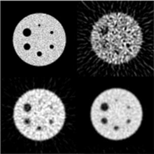 Fig. 4.5. : Effect of limited statistics on the quality of reconstructed images and lesion detection
The Jaszczak phantom with spheres insert consists of a water-filled cylindrical phantom containing uniform activity in which 6 cold spheres with diameters ranging from 9.5 to 31.8 mm are included. The reference image (top left) and reconstructed slices generated with 1 Mcounts (top right), 10 Mcounts (bottom left), and 50 Mcounts (bottom right) are shown.
The search for unified reconstruction algorithms led to the development of inverse Monte Carlo (IMC) reconstruction techniques (Floyd et al 1986). The authors used IMC to perform tomographic reconstruction for SPECT with simultaneous compensation for attenuation, scatter, and distance-dependent collimator resolution (see section 3.5.3).
4.3.4 Attenuation and scatter correction techniques
The presence of scatter and attenuation in the images limits the accuracy of activity quantification in emission computed tomography (Zaidi 1996b). With no corrections, the uncertainty could be as high as 50-100%. Monte Carlo calculations have been found to be powerful tools to quantify and correct for photon attenuation and scattering in nuclear medicine imaging since the user has the ability to separate the detected photons into their components: primary events, scatter events, contribution of down-scatter events, .. etc. Monte Carlo modelling thus allows a detailed investigation of the spatial and energy distribution of Compton scatter which would be difficult to perform using present experimental techniques, even with very good energy resolution detectors (Lowry and Cooper 1987).
Compton scattering effects in water on profiles of activity have been simulated (Logan and Bernstein 1983). The accuracy of experimental methodologies used for scatter fraction and scatter spatial distribution determination were evaluated using the Monte Carlo method (Acchiappati et al 1989). Barney et al (1991) developed an analytical simulation for single- and multiple-scattered annihilation photons in PET. The multiple-scatter model showed good agreement with Monte Carlo simulation of total object scatter. The authors also proposed a scatter correction method which uses the analytical simulation and exploits the inherent smoothness of the scatter distribution to account for three-dimensional effects in scatter distribution and object shape. Scatter components in PET divided into primaries, object scatter, gantry scatter and mixed scatter and their effects on the degradation of reconstructed images were also investigated (Adam et al 1996). Quantification of those components for a small animal PET prototype were also reported (Ziegler and Kuebler 1993). A Monte Carlo study of the acceptance to scattered events in a depth encoding large aperture camera made of position encoding blocks modified to have DOI resolution through a variation in the photopeak pulse height was performed (Moisan et al 1996). It was reported that the poorer discrimination of object scatters with depth sensitive blocks does not lead to a dramatic increase of the scatter fraction.
Levin et al (1995) developed a correction method that uses the 3D reconstructed image volume as the source intensity distribution for a photon-tracking Monte Carlo simulation. The history of each annihilation photon's interactions in the scattering medium is followed, and the sinograms for the scattered and unscattered photon pairs are generated in a simulated 3D PET acquisition. The calculated scatter contribution is used to correct the original data set. Monte Carlo techniques were also used to estimate 'best possible' weighting functions for different energy-based scatter correction schemes and to examine the optimal number of energy windows for both NaI(Tl) and BGO scintillators (Haynor et al 1997).
4.3.5 Dosimetry and treatment planning
There is no doubt that the area where early Monte Carlo calculations in the field have been performed is dosimetry modelling and computations (Andreo 1991). The approach adopted by the Medical Internal Radiation Dose (MIRD) committee of the Society of Nuclear Medicine was published as different pamphlets in a series of supplements to the Journal of Nuclear Medicine. Some of these pamphlets made extensive use of Monte Carlo calculations to derive specific absorbed fractions for electron and photon sources uniformly distributed in organs of mathematical phantoms. In particular, calculation of absorbed fractions for positron emitters relevant to neurologic studies were reported by Bice et al (1985). Interest in Monte Carlo-based dose calculations with b-emitters has been revived with the application of radiolabelled monoclonal antibodies to radioimmunotherapy (RIT).
Currently, the preferred strategy is personalised human dosimetry with radiolabelled antibodies and this approach may become routinely employed clinically. The dose distribution pattern is often calculated by generalising a point source dose distribution (Akabani et al 1997), but direct calculation by Monte Carlo techniques is also frequently reported because it allows media of inhomogeneous density to be considered (Tagesson et al 1996, Furhang et al 1996). The development of a 3D treatment planner based on SPECT/PET imaging is an area of considerable research interest and several dose calculation algorithms have been developed. Fig. 4.6 lists the essential steps required in developing a 3D treatment planning program for RIT. Projection data acquired from an emission tomographic imaging system are processed to reconstruct transverse section images which yields a count density map of source regions in the body. This count density is converted to an activity map using the sensitivity derived from a calibration phantom. In the final step, this activity distribution is converted to a dose rate or dose map by convolving the activity distribution with dose point kernels or by direct Monte Carlo calculations. To elaborate a treatment plan for an individual patient, prospective dose estimates can be made by using a tracer activity of radiolabelled antibody to obtain biodistribution information prior to administration of a larger therapeutic activity. The clinical implementability of treatment planning algorithms will depend to a significant extent on the time required to generate absorbed dose estimates for a particular patient.
 Fig 4.6. : Diagram showing the essential steps required in developing a three-dimensional internal dosimetry program based on quantitative positron emission tomography
4.3.6 Pharmacokinetic modelling
A few applications of Monte Carlo techniques have been reported in the field of pharmacokinetic modelling. Casciari et al (1995) developed a compartmental model of [F-18] fluoromisonidazole transport and metabolism to compute the volume average kappa in tissue regions from [F-18] fluoromisonidazole PET time-activity data and characterised it using Monte Carlo simulations and PET time-activity data. This model was able to accurately determine kappa for a variety of computer generated time-activity curves including those for hypothetical heterogeneous and poorly perfused tissue regions. Compartmental models allow also the in vivo analysis of radioligand binding to receptor sites in the human brain. Benzodiazepine receptor binding was studied using a three-compartmental model (Millet et al 1996). The validity of the results of the coefficient of variation of each parameter were verified with statistical results provided by Monte Carlo simulation. A simplified approach involving linear-regression straight-line parameter fitting of dynamic scan data was developed for both specific and non-specific models (Thie et al 1997). Monte-Carlo simulations were used to evaluate parameter standard deviations, due to data noise, and much smaller noise-induced biases. The authors reported good agreement between regression and traditional methods.
4.4 Monte Carlo computer codes
Many Monte Carlo programs have been in use in the field of nuclear imaging and internal dosimetry with many of them available in the public domain (Andreo 1991, Zaidi 1999a). The EGS4 code (Nelson 1986) represents actually the state of the art of radiation transport simulation in medical radiation physics because it is very flexible, well-documented and extensively tested. The GEANT package (Brun et al 1994) was originally designed for high energy physics experiments, but has found applications also outside this domain in the areas of medical and biological sciences, radiation protection and astronautics. MCNP is a general-purpose Monte Carlo code that can be used for neutron, photon, electron, or coupled neutron/photon/electron transport (Briesmeister 1997). Table 4.1 lists widely used Monte Carlo codes together with a short description of their key features. Those Monte Carlo software packages are excellent research tools and many of them could be freely obtained. However, Such programs tend to be powerful and poorly documented. Therefore, it might take a long time to become familiar with and they are usually not free of bugs. Moreover, the simulation package must be integrated in the local software environment. For that purpose, slight modifications may be necessary, which requires detailed knowledge of the package.
Many other simulation packages developed mainly for nuclear medical imaging research have been described in the literature. This includes codes designed to model projection data for simulated SPECT (Ljungberg and Strand 1989, Smith et al 1993), PET (Thompson et al 1992, Zaidi et al 1999a, Castiglioni et al 1999) or both imaging modalities (Harrison et al 1993). Some of these codes are based on existing simulation packages mentioned above (EGS4, MCNP, GEANT). For a detailed description of these codes, the reader is refereed to the excellent book by Ljungberg et al (1998) or the recent review by Zaidi (1999a).
| Table 4.1. : Key features of Monte Carlo codes used in simulation of nuclear medicine imaging systems |
| MC code |
General description |
| EGS4(Nelson et al 1985) |
Coupled photons/electrons transport in any material through user specified geometries. Simulation of imaging systems not specifically included and requires an extensive amount of user programming in Mortran. |
| ITS including TIGER CYLTRAN and ACCEPT (Halbleib et al 1992) |
Coupled photons/electrons transport in any material through slabs, cylinders or combinatorial. Simulation of imaging systems not specifically included and requires an extensive amount of user programming in Fortran. |
| MCNP(Briesmeister 1997) |
Coupled neutrons/photons/electrons transport in any material through user generalised geometry. Simulation of imaging systems not specifically included and requires an extensive amount of user programming in Fortran. |
| GEANT (Brun et al 1994) |
Coupled photons/electrons transport in any material through combinatorial geometry. Simulation of imaging systems not specifically included and requires an extensive amount of user programming in Fortran. |
| SIMSET(Harrison et al 1993) |
Photons transport in any material through voxel-based phantoms. Simulation of SPECT and PET imaging systems included. User modules written in C could be linked. |
| SIMIND(Ljungberg and Strand 1989) |
Photons transport in any material through voxel-based phantoms. Simulation of SPECT imaging systems included. User modules written in Fortran could be linked. |
| SIMSPECT(Yanch et al 1993) |
Coupled photons/electrons transport in any material through voxel-based phantoms. Simulation of SPECT imaging systems included. User modules written in Fortran/C could be linked. |
| MCMATV (Smith et al 1993) |
Photons transport in any material through voxel-based phantoms. Simulation of SPECT imaging systems included. User modules written in Fortran could be linked. |
| PETSIM(Thompson et al 1992) |
Photons transport in any material through shape-based phantoms. Simulation of PET imaging systems included. User modules written in Fortran could be linked. |
| EIDOLON (Zaidi et al 1998, 1999a) |
Photons transport in any material through source-based or voxel-based phantoms. Simulation of 3D PET imaging systems included. User modules written in C/Objective-C could be linked. |
| PET-EGS(Castiglioni et al 1999) |
Photons transport in any material through source-based or voxel-based phantoms. Simulation of 3D PET imaging systems included. User modules written in Fortran could be linked. |
7. Scatter Correction in 3D PET
One of the obstacles to the use of volume-imaging PET scanners is the increase in the scatter fraction which influences the sensitivity and represents more than 30% of the data acquired in 3D mode. The inclusion of Compton-scattered events degrade image quality and can seriously reduce diagnostic accuracy. In addition to a decrease in the image contrast, events may also appear in regions of the image where there is no activity (e.g. outside the patient). Scattered photons originate from the whole attenuating medium, including the imaging table and the PET tomograph itself. Implicit in all scatter correction methods in nuclear imaging is the existence of some complementary degradation model describing the nature and processes giving rise to detected scattered events. The general lack of theoretical connection between the degradation and correction models raises several important questions about the status of the fate of scattered events and the formulation of the required scatter correction models. The problem of scatter correction is of paramount importance in high-resolution PET imaging in which the scatter degradation features become more complex. The issue of scatter detection, modelling and correction are addressed in this chapter with the aim to exploit the achieved performance and accuracy of the Monte Carlo simulation package for this purpose.
7.1 The problem of Compton scatter
The fundamental information in PET is the distribution of a positron-emitting radiopharmaceutical as a function of position, direction and energy. Functionals of this distribution are measured experimentally by the imaging system. The transport of annihilation photons is described by the integro-differential Boltzmann equation which is the governing equation for a given monoenergetic, isotropic source of photons and a scattering medium. The differential part describes the generation, propagation and attenuation of photons. The integral part describes the scattering of photons as an integral over direction and energy. The Boltzmann equation describes the evolution of the spatial and angular distribution of photons with respect to time resulting from the generation, propagation, attenuation and scattering of photons within the medium. This equation is difficult to solve because of the scatter integral and the size of the problem when discretised. Many techniques deal with the scatter integral by discretely considering successive orders of scattering.
The probability of Compton scattering is given by the Klein-Nishina equation, which gives the differential scattering cross section  as a function of scattering angle q (Klein and Nishina 1929):
 |
(7.1) |
where  , E is the energy of the incident photon, and re the classical radius of the electron given by Eq. (2.5) in chapter 2. This equation was extensively used to build appropriate scatter models to correct for this effect in PET imaging. Since all unscattered events have 511 keV before scattering, a=1 for the first scatter. Therefore, the differential Compton scattering cross section relative to that for unscattered annihilation photons is:
 |
(7.2) |
The expression (7.2) gives the differential scattering probability. The integral of this from 0° to any angle gives the integral cross section. The integral gives information about what fraction of scattered photons will be scattered into a cone with a given half-angle. The theoretical angular and energy distributions of Compton-scattered photons are plotted as a function of the scattering angle and energy, respectively, in Fig. 7.1 for an initial energy of 511 keV. It illustrates relatively that small angle scattering is more likely than large angle scattering and that the most probable scattering angle is located around 35°. Note the excellent agreement between the theoretical distributions and those obtained by Monte Carlo calculations (Fig. 5.3).
7.2 Scatter components in 3D PET
There is no consensus in the literature on how to classify the detected coincidences in PET. We adopted a classification which distinguishes between a fixed tomograph-dependent component and a variable object-dependent component (Adam et al 1996). Unlike related studies, the annihilation photons were not restricted to single scattering, therefore the multiple scatter component was fully considered. By considering that scatter in the imaging table and tomograph gantry is negligible, four distinct classes can be distinguished (table 7.1) :
-
primaries or unscattered events (T);
-
object scatter (scatter in the phantom or the patient) (So);
-
detector scatter (scatter in the crystals) (Sd);
-
mixed scatter (scatter in the object and the detectors) (Sm).
| Table 7.1. : Classification of detected coincidences according to the location of scattering processes |
 |
| Primary |
| Object |
| Detector |
| Object + Detector |
For example, if the first recorded photon is unscattered (Primary) and the second photon is scattered in the object (Object), then the coincidence is classified as object scatter. The measured projection data, p, of a PET tomograph can thus be written in the following form:
| Table 7.1. : Classification of detected coincidences according to the location of scattering processes |
 |
(7.3) |
The scatter components, So and Sd in this model, are assumed to be the result of independent processes which for So neglect subsequent Compton interactions of object scattered photons in the detectors. This is a valid assumption when such processes are weak or have negligible effects on the scatter distribution (Bentourkia et al 1995).
Many scatter correction methods estimate the scatter response function, srf, of the tomograph from the response to a line or point source. The dependence of srf on source depth in the object was reported to be weak by many authors (Barney et al 1991). Based on the above assumptions, the normalised overall srfxri(x) to a line source at a given location in an object corresponding to radial position xr in the projection is also given as the sum of three components:
 |
(7.4) |
where srfxri(x) are the individual position-dependent projection response functions for the intrinsic or geometric detector response (i = g), object scatter (i = o), and detector scatter (i = d). Their relative intensities are described by the scaling factors fi which represent the fraction of each component; obviously  . Since in our assumptions, scatter components are independent of each other, it turns out that the detector scatter component can be estimated from a measurement made with a line source in the absence of the scattering media.
Geometric detector response function. The geometric detector response function is formed by annihilation photons which have not interacted with the object and were detected on the basis of a single interaction in the block detectors. Such photons belong to the true component since they carry exact information about the location of the source and activity concentration in the object. Fig. 7.2 illustrates the different possibilities of interaction of annihilation photons with the block detector. Annihilation photons impinging on the block detector can be completely absorbed in the crystal of first interaction (case 1 and 5), be scattered in the primary crystal and either escape from the block detector (case 3 and 4) or be absorbed in a neighbouring crystal (case 2). When the energy deposited in the primary crystal is above the lower energy threshold, cases 1, 3, 4 and 5 contribute to the geometric detector response.
When the LOR passes through the centre of the tomograph's FOV, the primary detectors are parallel and the geometric detector response function, which is specified mainly by the physical dimensions of the detectors is triangular in shape (case 1). Detector overlap increases when the source is moved off centre, the consequence of which is that the shape of the geometric detector response function varies with source position in the FOV (case 5). The width of the geometric detector response function is defined by a set of parallel LORs crossing the source and connecting the coincident detectors. Other physical effects including positron range and non-collinearity of the annihilation photons, which contribute to the broadening of the distribution by amounts comparable to the detector geometric and scatter components, can be considered to be part of the detector scatter component with the current assumptions (Thompson et al 1992).
When the energies deposited in primary and secondary crystals are both greater than the LLT, the coincidence is in principle rejected (case 2). However, this is not obvious on real PET scanners. If the energy deposited in the primary detector is above the LLT and the energy deposited in the secondary detector is below the LLT or lost in the detector package, then the coincidence becomes part of the geometric detector response, which is well-positioned. Monte Carlo simulation studies on the ECAT 953B tomograph, showed that the relative amounts of events illustrated in Fig. 7.2 are: 61% for case 1, 25% for case 2, and 14% for cases 3 and 4 combined.
 Fig. 7.2. : Illustration of photon interaction schemes within the detector blocks
|
(case 1) photoelectric absorption depositing all the incident energy in the crystal of first interaction or primary detector;
(case 2) multiple-energy deposit in primary and secondary detectors;
(case 3) Compton forward scatter depositing a small amount of energy (E �LLT) in the primary detector;
(case 4) Compton backward scatter depositing a larger amount of energy (LLT �E < 511 keV) in the primary detector; and finally (case 5) geometric detector response for LORs off-centre
|
Object scatter. The object scatter component is formed by annihilation photons which have interacted in the object by coherent or incoherent (mainly) processes (99.7% at 511 keV for H2O). Fig. 7.3 is a schematic representation of single and multiple object scatter. The object scatter distribution is object-dependent and depends on the size, depth, shape and composition of the media around the source. When the source is located at the centre of a uniform cylindrical phantom, the attenuation path lengths are symmetrically distributed, and therefore the object scatter distribution is expected to be symmetric about the centre of the object. When the source moves laterally towards the edge of the object, the asymmetry of the distribution increases progressively. The outer wing corresponds to the side with smaller photon path lengths in the object and has therefore a lower slope. The same effect results in a decrease of the amplitude of the object scatter across the FOV (Bentourkia et al 1995).
 Fig. 7.3. : Schematic diagram of the origin and shape of object scatter component estimated from measurements in a cylindrical phantom using a centered line source
Both single and multiple scatter are illustrated.
Detector scatter. The detector scatter consists of photons which have interacted within the block detectors by Compton scattering (53% at 511 keV for BGO) or by Rayleigh scattering (6% at 511 keV for BGO). It characterises the detection system and is dependent upon the energy discrimination threshold. Latest generation high-resolution PET tomographs are often made with long narrow detectors to increase detection efficiency and spatial resolution. However, the narrower the detectors, the greater the spillage of annihilation photons from primary to secondary detectors in the block. The effect of annihilation photon spillage is illustrated by case 2 in Fig. 7.2, where the photon deposits a small amount of energy below the lower energy threshold in the detector of first interaction and the rest is deposited in a neighbouring secondary detector. As shown in Fig. 7.4, the detector scatter contribution is confined to a narrow distribution around the primary detector due to the high density of the detector material (e.g. BGO). Detector scatter has therefore a negligible effect on the overall response function and has been ignored in medium- and low-resolution scanners. However, it has received considerable attention in high-resolution (e.g. small animal) PET scanners (Bentourkia et al 1995).
Mixed scatter. The mixed scatter is due to photons that are scattered in both the object and the block detectors. Consequently, the projections look like the projections of the object scatter convolved with the detector scatter distribution function, leading to nearly the same shape of the projections as for the object scatter, but with a smaller amplitude.
Fig. 7.5 shows projection response functions estimated with a line source at the centre of the FOV in air and in a 20 cm diameter water-filled cylinder. It is clear that the boundary (at -10 cm, +10 cm) of the object has no influence on the scatter profile. The profile from the 3D measurement, in particular, demonstrates how well defined the scatter portion of the curve is outside the object, and this has been the driving force to develop scatter correction methods based on fitting analytical functions to the recorded emission data outside the object being studied. As expected, the trues component shows a very narrow distribution whose width may be related to the spatial resolution of the scanner. Object scatter is a broad distribution and can be described fairly well by a monoexponential having low slope values. On the other hand, detector scatter is a narrow distribution squeezed to the neighbourhood of the source location in the FOV. The intensity and shape of this component should in principle be the same for measurements made with the source in air or in the water-filled phantom. However, for complex geometries and clinical studies, accurate estimation of detector scatter component may be difficult since it is masked by object scatter. This makes estimation of this component from measurements in air unavoidable.
 Fig. 7.4. : Schematic diagram of the origin and shape of the detector scatter component estimated from a measurement in air using a line source
 Fig. 7.5. : Illustration of the response functions normalised to the maximum amplitude for a line source at the centre of the FOV
The profiles in air and at the centre of a water-filled cylinder (R=10 cm) are summed over all projection angles showing trues, object and detector scatter components as obtained by Monte Carlo simulations.
7.3 Scatter modelling in 3D PET
Over the last two decades, many methods have been developed for the purpose of reducing the resultant degradation of image contrast and loss of quantitative accuracy. Some scatter compensation methods incorporate scatter in the transition matrix or point-spread function during iterative reconstruction. It has been shown that this can lead to highly quantitative accuracy (Floyd et al 1986, Frey and Tsui 1993, Ollinger 1996) and improved signal-to-noise ratio in the reconstructed images (Beekman et al 1997b).
Accurate simulation of scatter in PET projection data is computationally extremely demanding for activity distributions in non-uniform dense media. A complicating factor is that the scatter response is different for every point in the object to be imaged. Various methods for tackling this problem have been proposed. These methods require information about the attenuation map of the patient and can be divided roughly into two classes:
-
The first class of methods uses Monte Carlo simulations (Floyd et al 1986) to compute the transition matrix which represents the mapping from the activity distribution onto the projections. Monte Carlo simulation can readily handle complex activity distributions and non-uniform media. Unfortunately, hundreds of Gbytes up to several Tbytes of memory are required to store the complete non-sparse transition matrix when the fully 3D Monte Carlo matrix approach is used, and it can take several weeks to generate the full matrix on a state-of-the-art workstation. In addition, the procedure has to be repeated for each patient. Analytical scatter models, based on integration of the Klein-Nishina (K-N) equation (Riauka et al 1996), have practical disadvantages which are similar to those of Monte Carlo-based methods.
-
The second class of methods, which includes anatomy-dependent scatter in the reconstruction, first calculates and stores in tables the scatter responses of point sources behind slabs for a range of thicknesses, and then tunes these responses to various object shapes with uniform density (Frey and Tsui 1993). This method is referred to as slab-derived scatter estimation (SDSE). A table occupying only a few Mbytes of memory is sufficient to represent this scatter model for fully 3D SPECT reconstruction (Beekman et al 1997a). A fully 3D reconstruction of a 99mTc cardiac study based on SDSE can be performed in only a few minutes on a state-of-the-art single processor workstation. A disadvantage of SDSE compared with matrices generated by Monte Carlo simulation or Klein-Nishina integration is that it cannot accurately include the effects of the non-uniform attenuation map of the emitting object. So far, only a few rough adaptations have been proposed to improve the accuracy of SDSE in non-uniform objects (Frey and Tsui 1994, Beekman et al 1997a).
While Monte Carlo simulation is the gold standard for simulating PET data, there are situations where it is not suitable due to the large computational burden. In these cases, it is desirable to develop quick, accurate methods for modelling the projection data. In this section, we describe a simple method for analytically estimating the scatter component in the projection data for a known source and uniform attenuating medium as a scatter model. Two such applications are forward-projection of the data for use in iterative reconstruction methods for scatter compensation and the analytic generation of simulated projection data for applications requiring large numbers of data sets of different projection data such as observer studies or training of neural networks. However, Monte Carlo simulation is invaluable in developing and evaluating these scatter models.
Considering the requirements of these typical applications, the motivation for developing scatter models becomes more clear. For example, iterative reconstruction-based scatter compensation requires to compute the srf at each point in the attenuator with respect to each projection view. Both the computation time and the memory required to store the data are impractical, especially for 3D reconstruction. Moreover, the srf is generally different for every point in the object to be imaged. Inclusion of the effects of non-uniformity of the attenuator in the scatter model is still computationally very demanding. To speed up simulations, approximate methods have been suggested which are very accurate in the case of uniform media (Beekman et al 1997a, Frey and Tsui 1993), but still have problems with non-uniform objects. Monte Carlo simulation allows to include very accurately the effects of non-uniformity in the srf . However, almost noise free projection data are desired in order to minimise statistical errors in model-based iterative reconstruction.
The other application where scatter models are important is the generation of projection data for applications requiring large numbers of data sets like studies involving receiver operating characteristic (ROC) analysis and developing training sets for neural networks. In both applications, it is desirable to generate a large number of data sets having Poisson-distributed noise from different source and attenuator configurations. Using Monte Carlo simulation to generate these data sets is prohibitive. For example, generating a noise-free 3D data set with Monte Carlo simulation typically takes of the order of weeks of computing time.
While Monte Carlo simulation is not practical as a method of simulating projection data in these cases, it is an indispensable tool in developing scatter models. The process of developing scatter models occurs in four stages: characterisation, development, validation and evaluation.
-
Characterisation. Monte Carlo simulation is used to study the srf in various phantoms to get a feeling and a clear idea of how parameters such as source position, attenuating medium shape and composition and detector energy resolution affect the srf.
-
Development. A scatter model can be developed based on the intuition gained in these studies. At this stage, Monte Carlo may again prove valuable in estimating parameters necessary for the scatter model. After developing the model, it is important to validate it.
-
Validation. The validation process involves comparing the predictions of the model, for example the srf and projection data for various phantoms, with those from either Monte Carlo simulations or direct experimental measurements. Monte Carlo simulation are often preferred to direct measurements because of the ability to simply and accurately control and know the phantom geometry and source position, as well as the ability to separate scattered and unscattered events.
-
Evaluation. The final step is the evaluation of the scatter model in terms of the purpose for which it was developed. For example, for the case of iterative reconstruction-based scatter compensation, this includes evaluating the effectiveness of the method in comparison with other scatter compensation methods.
Many investigators used Monte Carlo techniques to study the srf (Frey and Tsui 1990, Ljungberg and Strand 1990, Barney et al 1991). However, even with the use of variance reduction techniques, these simulations require large amounts of computer time (Zaidi et al 1998), and the simulation of the srf for each patient is impractical.
Beekman et al (1999) reported an accurate method for transforming the response of a distribution in a uniform object into the response of the same distribution in a non-uniform object. An efficient and accurate method has been presented for estimating scatter distribution in projections from objects with non-uniform mass density by using two simulated projections which include only first-order scatter. These two Monte Carlo simulated projections are generated in such a way that the noise level is low because the collimator is modelled analytically after probabilistic photon scatter modelling has been performed (Beekman et al 1999). However, the time needed to calculate correction maps for transforming a response from uniform to non-uniform objects may be somewhat too long for routine clinical implementation in iterative scatter correction, especially when the correction maps are calculated for all projection angles and each iteration anew. The use of only one order of scatter was sufficient for an accurate calculation of the correction factors needed to transform the scatter response. Since the computation time typically increases linearly with the number of scatter orders, it still remains much shorter than with straightforward Monte Carlo simulation.
In this work, a simple parametrization of the scatter distribution function is performed by fitting simulated response functions to a line source with mono-exponential kernels. The scatter fractions were also parametrised by a simple fitting function. The results are presented in the following sections.
7.3.1 Scatter distribution functions
It has been shown (Fig. 7.5) that the projections of a line source placed in a uniform water-filled cylinder are dominated in the wings by the object scatter and in the peak by the unscattered photons. As expected, the object scatter is fairly well described by the monoexponential functions. The detector scatter, on the other hand, is closely located around the primary peak. This observation seems reasonable, since the point of interaction of a photon scattered in the crystal is closer to the centroid of interaction than that of a photon scattered in the object, leading to a smaller deviation of the scattered photons. Since the detector scatter has no significant contribution to the wings of the scatter distribution function, it can be added to the unscattered component.
This discussion remains valid, when the line source is shifted out of the symmetry centre. The amplitude of the short side of the projection, compared to that of the symmetrical case is increased, since the path length of the photons through the phantom becomes shorter, whereas the amplitude of the long side is decreased, due to a longer pathway through the attenuating medium. The wings of the scatter distribution functions are still well parametrised by mono-exponentials, but with different parameters for the left and the right side. The data presented reveal that the amount of multiple scatter is at least 10-15% of the scattered photons. The rationale of several scatter correction algorithms is to consider the multiple scatter by rescaling the single scatter component. This approach seems to be questionable in view of the results obtained by the Monte Carlo calculations. Obviously, a rescaling does not change the shape of the different scatter components.
Fig. 7.6 shows scatter distribution functions when the line source is located at the centre of the FOV (left) and displaced 5 cm radially off-centre (right). The projections for the line source at the centre are symmetrical and were summed over all projection angles. This is not the case when the source is moved off-centre. In this case, a profile of a single angular view was used. The scatter function kernel was assumed to be mono-exponential with exponent decreasing linearly as a function of the radial position. A linear regression analysis on the wings of the log plot of the projection data was used to estimate the slope, a (in units of cm-1). The data in the extreme bins of the projection were excluded to avoid edge effects.
| Fig. 7.6. : Illustration of the scatter response functions when the line source is located at the centre of a water-filled cylindrical phantom (left) and displaced 5 cm radially (right) |
 |
 |
The projections for the line source placed at the centre of the FOV are symmetrical and were summed over all projection angles.
The scatter function was examined with respect to three parameters: (i) variation in lower level threshold setting; (ii) variation in radial position of the line source within the cylindrical phantom; and (iii) variation in the diameter of the cylindrical phantom. For the case when the line source was located at the centre of the cylinder, table 7.2 shows a progressive increase in the slope of the scatter function from 0.037 cm-1 to 0.099 cm-1 with increasing lower level threshold. This is consistent with the fact that the scatter tails are less pronounced when the lower level threshold is increased. For comparison purposes, the measured values of the srf slopes for the ECAT 953B are also shown. Note that when the line source was located at the centre of the cylinder and the LLT was varied, the source is in the same location in the sinograms at all projections. This allows to estimate a and its standard deviation from all 2D radial measurements. When the line source was translated radially along the x-axis of the scanner, only the projection corresponding to the first view (F = 0) was considered. The effect of increasing the axial acceptance angle of the sinograms up to dr = 12 was negligible. A good agreement between measured and simulated data was observed except for a LLT setting of 250 keV.
| Table 7.2. : Measured and simulated values of a (in cm-1), the slope of the scatter response function exp(-ar) for different lower level energy window settings obtained by linear regression analysis |
| Lower energy window setting (keV) |
| 250 |
| 300 |
| 350 |
| 380 |
| 400 |
Table 7.3 shows the variation of a as a function of the radial displacement. The slope of the scatter function is seen to increase on one side of the peak while decreasing on the other side. A variation by a factor of over two is also observed. As the line source is moved radially, the slope decreases (i.e. an increase in scatter) outside the object up to some limit, while the slope increases inside the object (i.e. a decrease in scatter), which is consistent with the observations made by Bailey and Meikle (1994). By observing the profiles of the line source at different radial locations, it was noticed that many scattered events are still recorded even when the line source is placed just inside the edge of the cylinder (9.5 cm).
| Table 7.3. : Simulated and measured variation of a (in cm-1), the slope of the scatter function exp(-ar) for either side of the log profile at different radial locations |
| Radial distance from centre (cm) |
| 0 |
| 5 |
| 7.5 |
| 9.5 |
All simulations were made with a lower energy window threshold of 380 keV.
On the basis of the results presented in the preceding tables, the effect of the size of the cylinder on the spatial variation of scatter estimation was further investigated. The variation of a as a function of the radius of the cylindrical phantom is illustrated in table 7.4. It can be seen that the slope increases with increasing the size of the cylinder on both sides of the peak. This parameter changes by a factor of around two when increasing the radius of the cylinder from 5 cm to 20 cm.
| Table 7.4. : Variation of a (in cm-1), the slope of the scatter function exp(-ar) for different sizes of the water-filled cylinder serving as scattering medium |
| Radius of the cylinder (cm) |
slope of the srf (cm-1) |
| 5 |
0.069 |
| 8 |
0.074 |
| 10 |
0.084 |
| 12 |
0.090 |
| 15 |
0.101 |
| 18 |
0.119 |
| 20 |
0.129 |
All simulations were made with a lower energy window threshold of 380 keV.
7.3.2 Scatter fractions
The variation of the scatter fraction (SF) was investigated in the same way as the scatter distribution function. However, in addition to the line source geometry, the variation of the scatter fraction in a uniform cylindrical phantom as a function of its size and for three lower energy thresholds (250, 380 and 450 keV) was also studied. The scatter fraction is estimated directly from the results of the Monte Carlo simulation as the ratio between scattered and total coincidences. Fig. 7.7 shows the SF versus the radius R of the cylindrical phantom. Obviously, SF(R) increases with increasing R. To fit the data, a simple function was derived  . As reported by Adam et al (1996), this function fits the scatter fraction of a uniform activity distribution in cylindrical phantoms (Fig. 7.7), as well as centred (Fig. 7.8) and a 5 cm off-centred line sources (Fig. 7.9) reasonably well, although some crude simplifying assumptions have been made for the derivation of this function. This simple formula for the scatter fraction was derived by assuming that the probability of a photon not to be scattered is proportional to
  (where x is the pathlength of the photon). The same assumption is valid for the second photon of the pair, leading to a probability for both photons not to be scattered proportional to
  . In the case of a centred line source, the total length through the cylinder is always twice the radius R. Thus, the probability of two coincident photons not to be scattered is proportional to
  . The probability of two coincident photons to be scattered could then be obtained since the two probabilities are complementary. Moreover, the percentage of Compton interactions in the object consist of more than 99.7% at 511 keV for H2O which renders the number of interactions by photoelectric absorption negligible. The second argument is that for the majority of detected scattered events, only one of the two annihilation photons undergoes a single Compton interaction. The single scatter distribution was reported to consist of more than 75% of detected scattered events (Ollinger 1996). The fit function is therefore
  and the normalisation constraint that the limit for
  should be 1 is verified. This simple functional dependence for the scatter fraction was also assumed for homogeneously distributed activities.
 Fig. 7.7. : Monte Carlo calculations of the variation of the scatter fraction as a function of the radius R of the cylindrical phantoms for a homogeneous activity distribution for three different LLT settings
The fitted curves are also shown.
With increasing the lower energy discrimination level, the scatter fraction decreases. An increase of the energy threshold reduces the number of registered scattered coincidences, but it also decreases the sensitivity leading to a reduced number of true coincidences. As expected (and confirmed by Monte Carlo simulations), the largest effect is achieved for multiple scattered photons and photons that are scattered under a large angle.
 Fig. 7.8. : Monte Carlo calculations of the variation of the scatter fraction as a function of the radius R of the cylindrical phantom for a central line source for three different LLT settings
The fitted curves are also shown.
 Fig. 7.9. : Monte Carlo calculations of the variation of the scatter fraction as a function of the radius R of the cylindrical phantom for a line source 5 cm off-axis for three different LLT settings
The fitted curves are also shown.
It was observed that, for the same phantom size, the scatter fraction for a line source is always larger than that for a homogeneously distributed activity. The higher scatter fraction for a line source centred in the cylinder compared to a homogeneous activity distribution in the same cylinder can be explained as follows. For a line source, the two annihilation photons must always travel the maximum path length through the phantom, which is not the case for a homogeneously distributed activity. The activity distribution in cerebral scans can be considered as a mixture of both components. Consequently, its scatter fraction is between the two extremes. The scatter fraction for a non-uniformly attenuating medium in the thorax region (oncology clinical study described in section 7.6), compared to a cylindrical phantom with a comparable (similar) cross-section (R=15 cm), is larger than that for a homogeneously distributed activity, but smaller than that for a line source.
Better fitting was achieved using third order polynomials, however, preference was given to the simple parametrization presented above for both simplicity and reproducibility purposes. Since the function  fits the object scatter fraction for uniform activity distributions and line sources (centred and off-centre) in cylindrical shaped objects reasonably well (Figs. 7.7-7.9), it allows an estimation of the amount of object scatter for simple activity distributions. According to the definition presented in table 7.1, unscattered and detector scatter components are not indistinguishable until they enter the crystal volume since they are both not scattered in the object. This means that the detector scatter is correlated with the primaries and not with the object scatter, which was already assumed in other studies (Bentourkia et al 1995). Hence, the detector scatter becomes relevant for small objects, such as small animals, scanned on high-resolution scanners, when the object scatter fraction is very small (Ziegler and Kuebler 1993).
7.4 Overview of scatter correction approaches
Much research and development has been concentrated on the scatter compensation required for quantitative 3D PET. Increasingly sophisticated scatter correction procedures are under investigation, particularly those based on accurate scatter models, and iterative-based scatter compensation approaches. Monte Carlo methods give further insight and might in themselves offer a possible correction procedure.
The main difference among the correction methods is the way in which the scatter component in the selected energy window is estimated. The most reliable method to determine the actual amount of scatter in the image is physical modelling of the scatter process to resolve the observed energy spectrum into its unscattered and scattered components. By observing how accurately a scatter correction algorithm estimates the amount and distribution of scatter under conditions where it can be accurately measured or otherwise independently determined, it is possible to optimise scatter correction techniques. A number of scatter correction algorithms have been proposed in the literature. They fall into four broad categories (Bendriem and Townsend 1998):
-
Energy window-based approaches,
-
Convolution/deconvolution-based approaches,
-
Approaches based on direct estimation of scatter distribution.
-
Statistical reconstruction-based scatter compensation approaches.
Different versions of the above methods have been successfully implemented for 3D PET and are briefly discussed below.
7.4.1 Energy window-based approaches
Multiple energy window methods have been originally developed for SPECT and have been in use for more than 15 years (Zaidi 1996b). The development of 3D acquisition mode and improvements in the detector energy resolution have allowed the implementation of scatter correction based on the analysis of energy spectra. Several groups investigated the potential of acquiring data in two (Grootoonk et al 1996, Bendriem et al 1993), three (Shao et al 1994) and multiple (Bentourkia et al 1995) energy windows to develop corrections for scattering in 3D PET.
Two variants of dual-energy window techniques have been proposed: methods estimating the scatter component in the photopeak window from the events recorded in a lower energy window placed just below the photopeak and methods estimating the unscattered component in the photopeak window from the unscattered counts recorded in a high energy window in the upper portion of the photopeak. The dual energy window (DEW) technique (Grootoonk et al 1996) belongs to the former while the estimation of trues method (ETM) (Bendriem et al 1993) belongs to the latter.
In the practical implementation of the dual-energy window method on the ECAT 953B scanner, detected coincidence events are assigned to the upper energy (UE) window when both photons deposit energy between 380 keV and 850 keV, or to the lower energy (LE) window when one or both photons deposit within 200 keV and 380 keV (Grootoonk et al 1996). Both energy windows are assumed to contain object scattered and unscattered events. The coincidence events in both energy windows in each sinogram can be expressed as follows:
 |
(7.5a)
(7.5b) |
where unsc and sc refer to the unscattered and scattered components, respectively. These two equations contain four unknown parameters and so additional data are required to solve the system of equations and extract the unscattered components. Let us define Rsc as the ratio of scattered events and Runsc as the ratio of unscattered events detected in both windows:
 , ,  |
(7.6) |
Thus Eq. (7.5a and 7.5b) can be re-arranged to give the following expression for scattered events in the upper window:
 |
(7.7) |
UEunsc can then be obtained from equation (7.7) by subtracting UEsc from UE. The scaling parameters Rsc and Runsc are derived from measurements of the ratios of counts from line sources due to unscattered (measurements in air) and scattered events (measurements in a head-sized phantom) in the two energy windows, respectively.
The estimation of trues method (Bendriem et al 1993) consists in acquiring data simultaneously into two energy windows: a high window with a lower energy threshold higher than 511 keV and a regular acquisition window including the higher window. Therefore, both windows have the same upper energy threshold (UET) value. The hypothesis of this method is that the number of unscattered coincidences recorded in a given energy range depends on the energy settings of the window and the angle of incidence of the annihilation photons on the detector face. Hence, the unscattered component in the high energy window can be related to the unscattered coincidences in the standard wider window through a function of the energy settings, the radial position in the sinogram for a given LOR and the axial opening for a given radial position. This calibrating function is in principle independent of the source distribution. The unscattered component in the wide energy window can thus be calculated and subsequently subtracted from the data recorded in the regular window to produce a scattered sinogram. The unscattered component in the regular window is then obtained by smoothing that sinogram and subtracting it from the data recorded in the standard window.
The triple energy window method (Shao et al 1994) was suggested as an extension of the DEW technique. Coincidence events are recorded in three windows: two overlapping windows having the same UET settings (450 keV) located below the photopeak window and a regular window centred on the photopeak and adjacent to the low windows. A calibrating function that accounts for the distribution of scattered coincidences at low energies is obtained by calculating the ratio of the coincidence events recorded in both low energy windows for the scanned object and for a homogeneous uniform cylinder. The scatter component in the standard acquisition window is then estimated from the calibrating function and the narrower low energy window.
The multispectral method is based on the acquisition of data in a very large number (typically 256) of windows of the same energy width (16x16 energy values for the two coincident photons). The spatial distribution of scattered and unscattered components in each window can be adjusted using simple mono-exponential functions (Bentourkia et al 1995). The method presents the advantage of increased sensitivity due to smaller rejection of detected coincidence events (~10%) since the position of the scattered photons in the detectors can be restored. The statistical noise in each window and the necessity to accommodate the acquisition hardware with the required electronic boards to allow acquisition in multiple windows remain the major obstacles for implementation of the method on commercial PET scanners.
7.4.2 Convolution-deconvolution based approaches
Techniques based on convolution or deconvolution estimate the distribution of scatter from the standard photopeak data. The scatter fraction (SF) which gives an indication about the expected amount of scatter and the scatter response function (srf) which defines the spatial distribution of scatter in the photopeak data are usually the two parameters required for estimation of scatter component and need to be determined a priori. A pure additive model of the imaging system is generally assumed where the recorded data are composed of an unscattered and a scattered component plus a noise term due to statistical fluctuations, and can be written in the following form:
 |
(7.8) |
where po are the observed data, pu and ps are the unscattered and scattered components respectively, and  is the noise term. The problem to be addressed consists in estimating the unscattered distribution (pu) from the measured data (po) contaminated by scatter, or alternatively estimate the scattered component (ps) and then derive pu. The proposed methods differ in the way the scatter function is defined.
The convolution-subtraction (CVS) technique developed for 3D PET (Bailey and Meikle 1994) operates directly on projection data (pre-reconstruction correction) and is based on the assumption that the convolution of the source distribution with the srf gives an estimate of the scatter component. Two assumptions have been made: the stationary and nonstationary assumptions. In the stationary assumption, the scatter is assumed to be analytically defined and not dependent on the object, activity distribution, etc. The nonstationary assumption overcomes this problem by taking into consideration the dependence of scatter upon source locations, object size, detector angle, etc. Using the stationary assumption, the scatter component can be related to the unscattered component by the convolution relation:
 |
(7.9) |
where  denotes the convolution operator. The scatter estimate (ps) is then subtracted from the measured data (po) after scaling by an appropriate scatter fraction (SF). The process can be repeated iteratively with each step using the previous estimate of the scatter-free distribution as input to the scatter estimation (Bailey and Meikle 1994). The observed data are used as a first approximation to the unscattered distribution (pu) and the process is repeated iteratively with each step using the previous estimate of the scatter-free distribution as input to the scatter estimation:
 |
(7.10) |
where the '' indicates that the parameter is a rough estimate of the scatter and n is the iteration number. The rationale is that with each iteration, the input to the scatter estimation step more closely approximates pu. It was also suggested to use a damping factor to prevent oscillation in the result.
The convolution-subtraction approach can also be applied to reconstructed images (post-reconstruction). In this case, the scatter estimates are reconstructed and then subtracted from the non-corrected reconstructed images of the acquired data (Lercher and Wienhard 1994).
Scattered photons degrade the point-spread function (PSF) of the PET camera; the long tails of the PSF are mainly due to scatter. Thus, deconvolution methods which correct the images for the PSF will also, implicitly correct for scatter. In general, the PSF will act as a low-pass filter. Deconvolution will restore the high-frequency contents of the signal emitted by the object, at least as long as they have not yet been completely removed by PSF. Not only the high-frequencies in the signal are restored, but also the high-frequency noise is amplified, which in turn can degrade the image again. Therefore, the restoration filter is often combined with a low-pass filter that balances that image improvement by deconvolution and its degradation due to amplification of noise. Well known examples of these filters are the Wiener and Metz filters. Links et al (1992) studied the use of two-dimensional Fourier filtering to simultaneously increase quantitative recovery and reduce noise. The filter is based on the inversion of the scanner's measured transfer function, coupled with high-frequency roll-off. In phantom studies, they found improvements in both 'hot' and 'cold' sphere quantification. Fourier-based image restoration filtering is thus capable of improving both accuracy and precision in PET.
The curve fitting approach is based on the hypothesis that detected events assigned to LORs outside of the source object must have scattered and that the scatter distribution corresponds to a low-frequency component that is relatively insensitive to the source distribution. Estimation of the unscattered component can thus be performed in three successive steps: (i) fitting the activity outside the source object with an analytical function (e.g. Gaussian), (ii) interpolating the fit inside the object, and (iii) subtracting the scatter component from the observed data (Cherry and Huang 1995). The accuracy of this class of scatter correction methods depends on how accurately the scatter components can be estimated. The appropriate choice of a set of parameters which should be optimised for each PET scanner and for different radioactivity distributions is the dominant factor.
7.4.3 Approaches based on direct calculation of scatter distribution
This class of methods assume that the distribution of scattered events can be estimated accurately from the information contained in the emission and transmission data. For the majority of detected scattered events, only one of the two annihilation photons undergoes a single Compton interaction. The rationale of most of these methods is that the overall scatter distribution can be computed from the single scatter distribution (~75% of detected scattered events) and that this latter can be scaled to model the distribution of multiple-scattered events (Ollinger 1996). The multiple scatter distribution is generally modelled as an integral transformation of the single scatter distribution. The same approach can also be applied to scatter estimation in transmission imaging. Monte Carlo simulation studies of various phantom geometries demonstrated the accuracy of this method for fully 3D PET imaging by direct comparison of analytic calculations with Monte Carlo estimates (Barney et al 1991).
The model-based scatter correction method developed by Ollinger (1996) uses a transmission scan, an emission scan, the physics of Compton scatter, and a mathematical model of the scanner in a forward calculation of the number of events for which one photon has undergone a single Compton interaction. A single-scatter simulation technique for scatter correction where the mean scatter contribution to the net true coincidence data is estimated by simulating radiation transport through the object was also suggested and validated using human and chest phantom studies (Watson et al 1997). However, the above methods do not correct for scatter from outside the field-of-view. This effect can be directly taken into account by acquiring short, auxiliary scans adjacent to the axial volume being investigated. This implicitly assumes that the distribution of scatter from outside the FOV has the same shape as that of scatter from inside the FOV. These extra data are naturally available in whole-body imaging. However, this method is impractical for isotopes with a short half-life or rapid uptake relative to the scanning interval.
The true scatter component (being an experimentally impossible measurement) can be accurately estimated using rigorous Monte Carlo simulations. Given a known radioactive source distribution and density of the object, Monte Carlo techniques allow detected events to be classified into unscattered and scattered events and the scatter component to be determined in an independent way. However, the source and scattering geometry is generally not known in clinical studies. Levin et al (1995) used filtered-backprojection reconstructions as an estimate of the true source distribution. This input image is then treated as a 3D source intensity distribution for a photon-tracking simulation. The number of counts in each pixel of the image is assumed to represent the isotope concentration at that location. The image volume planes are then stacked and placed at the desired position in the simulated scanner geometry assuming a common axis. The program then follows the history of each photon and its interactions in the scattering medium and traces escaping photons in the block detectors in a simulated 3D PET acquisition. The distributions of scattered and total events are calculated and sorted into their respective sinograms. The scatter component is equal to the difference between measured data and the scaled and smoothed scatter component. To reduce the calculation time, coarser sampling of the image volume over regions equivalent to 4x4 pixels was adopted assuming that the Compton scatter distribution varies slowly over the object. For obvious reasons, the implemented method do not correct for scatter from outside the field-of-view and further refinements of the technique were required to take this effect into account as described in section 7.5.1.
7.4.4 Iterative reconstruction-based scatter correction approaches
Improvement in computer speed and recent advances in acceleration of reconstruction algorithms (Hudson and Larkin 1994) have led to renewed interest in algorithms which incorporate scatter as part of the emission model. Iterative reconstruction-based scatter compensation has received considerable attention during the last decade. Earlier studies (Frey et al 1993, Beekman et al 1997b) indicate that when scatter is modelled in iterative reconstruction, higher contrast and lower noise can be obtained than when the technique of scatter subtraction is used. In addition, model-based iterative reconstruction does not require patient-dependent parametrization. Development of scatter models which can be incorporated in statistical reconstruction (e.g. ML-EM) of PET continues to be appealing, however, implementation must be efficient to be clinically applicable.
One of the requirements of this method is to compute the scatter response function at each point in the attenuator with respect to each projection view. An efficient algorithm for scatter estimation was recently described in which the spatial scatter distribution is implemented as a spatially invariant convolution for points of constant depth in tissue (Hutton and Baccarne 1998). The scatter estimate is weighted by a space-dependent build-up factor based on the measured attenuation in the body. This approach was validated by Monte Carlo simulation studies of a realistic thorax phantom.
The normal approach for implementation of a scatter model is to incorporate the scatter estimation directly in the transition matrix (aij), although efficiency has been improved by utilising a dual matrix approach (Kamphuis et al 1998) in which scatter is incorporated in the forward projection step only. In this case, aij is considerably larger than is necessary if only attenuation and geometric factors are included and computation is therefore slow since scatter is essentially recalculated and added each iteration. In the case of constant pre-calculated (or measured) scatter, for example, as in multi-energy window methods, this scatter estimate either can be subtracted directly from projections (pi) prior to reconstruction, or alternatively can be introduced in the denominator of the ML-EM equation (Eq. 7.11). This latter approach results in better noise properties than direct subtraction.
 |
(7.11) |
where Si is the scatter estimated on all projections. Hutton and Baccarne (1998) proposed that S can be estimated once, based on an estimate of the activity distribution obtained from Eq. (3.12) in chapter 3, with the final scatter-corrected result obtained by proceeding with Eq. (7.11). It is worth to point out that most of the research performed in this field is related to SPECT imaging. Further development and validation of this class of algorithms in 3D PET are still required.
7.5 Proposed scatter correction techniques
Accurate scatter correction is one of the major problems facing quantitative 3D PET. Simple and more sophisticated scatter correction techniques have their own advantages and drawbacks. Most of these methods attempt to estimate the scatter contamination and then remove it using either subtraction or deconvolution techniques. There have been a number of studies comparing these methods in SPECT and PET imaging (Ljungberg et al 1994; Townsend et al 1996; and others). The primary concerns affecting these methods are: (i) the scatter estimates may be inaccurate, leading to bias in the reconstructed image; and (ii) the scatter compensation is often accompanied by a substantial increase in statistical noise. In addition, many of the methods require estimating parameters that may change for each patient and imaging protocol. With the advent of faster computers and accelerated iterative reconstruction algorithms, different approaches to scatter compensation are receiving much attention.
As stated previously, one of the main motivations for developing the Eidolon simulation package is to use it in investigating scatter distribution and its effect on reconstructed images, as well as its application for development and evaluation of scatter correction methods. This tool has potential applications as a possible alternative to fastidious experimental measurements for studying scatter models and correction techniques. Also, it can be used to generate accurate, patient-specific, and spatially-varying scatter kernels for scatter correction in methods such as convolution-subtraction, and can also serve as an accurate forward projector in iterative reconstruction techniques. Moreover, if its execution time can be improved, this will render its routine application in a clinical environment viable.
This section presents the contributions made in the field of scatter correction in 3D PET. An improvement and extension to whole-body 3D imaging of a recently proposed method (Levin et al 1995) and a new scatter correction approach based on statistical reconstruction are proposed and evaluated against more common correction methods using Monte Carlo simulated data, experimental measurements and clinical studies.
7.5.1 Monte Carlo-based scatter correction (MCBSC)
The possibility of using Monte Carlo simulation to calculate and correct for Compton scatter in 3D PET was first suggested by Levin et al (1995). As proposed, the method uses as an estimate of the true distribution, the non-scatter corrected reconstructed 3D image volume for a simulated 3D PET acquisition, assuming that the number of events in each voxel accurately represents the number of annihilation photons originating at the corresponding location within the simulated body. Monte Carlo simulations requires as input the voxelised source distribution as well as the corresponding distribution of attenuation coefficients. The contours and attenuation coefficients of the different organs and tissues are obtained from a segmented transmission image derived from a short transmission scan.
The sinograms of simulated scattered and unscattered events are created and used to estimate the scatter distribution for any given plane. For obvious reasons, the Monte Carlo generated data sets have a lower number of events than the measured data sets. Scaling of the simulated scatter distribution is therefore required to normalise the statistics of the simulated and the measured data. This scale factor was calculated as the ratio between the uncorrected emission sinograms and the total simulated emission sinogram (unscattered + scattered). Correction for scatter is performed by subtracting the estimated scatter distribution,  , multiplied by the calculated scale factor from the measured emission data set according to:
 |
(7.12) |
where k is the ratio of total counts in the acquired data to the total counts in the simulated data. To reduce computation time, the authors proposed to use coarse sampling of the input emission and segmented transmission images. That is, a 128x128 image volume is resampled to 32x32 by grouping 16 pixels (4x4) in a single pixel. As proposed by Levin et al (1995), the reconstructed emission image used as input to the simulations was not pre-corrected for scatter. This results in an overestimation of the amount of scatter and blurring in the emission image due to miss-positioning of events. This standard method is refereed as MCBSC1 in this section. The authors claim that the negative systematic errors introduced by the inclusion of scatter in the input image are less relevant than the statistical noise in the data sets. Fig. 7.10 illustrates the basic principles of the standard method (MCBSC1).
 Fig. 7.10. : Flow-chart illustrating the basic principles of the original Monte Carlo-based scatter correction method (MCBSC1)
The limitations of the technique are also mentioned (in bold).
The contribution of scatter from out-of-FOV activity is particularly significant in 3D whole body scanning. To take this effect into account, activity from outside the FOV should be incorporated in the calculation of the scatter distribution. For this purpose, data from several bed positions should be made available as input to the Monte Carlo simulation. The effect of pre-correcting the projection data for scatter using an approximate method (e.g. CVS) was also investigated in this work. The data sets were pre-corrected for scatter with the CVS method and the reconstructed images are then used as input to the Monte Carlo simulator. This approach seems reasonable from the point-of-view of the physics of PET imaging and is refereed in what follows as MCBSC2 which can be distinguished from MCBSC1 by the modifications mentioned above. Fig. 7.11 illustrates the basic principles of the modified version of the algorithm (MCBSC2).
 Fig. 7.11. : Flow-chart illustrating the principles of the modified Monte Carlo-based scatter correction method (MCBSC2)
The modifications and improvements brought to the technique are outlined (in bold).
The effects of pre-correcting the first image estimate for scatter on the estimation of scatter distribution is illustrated in Fig. 7.12 for a clinical brain study. A representative plane of the Monte Carlo simulated scatter sinograms using as input reconstructed images not corrected for scatter (left), and the same plane of Monte Carlo simulated sinograms using as input reconstructed images corrected for scatter (middle) are shown. Normalised differences between both sinogram are also shown (right). Integral profiles of the simulated low statistics scatter sinogram planes showing small differences between the two distributions are also illustrated in Fig. 7.13.
 Fig. 7.12. : Clinical cerebral study showing a representative plane of the Monte Carlo simulated scatter sinograms using as input reconstructed images not corrected for scatter (left), and the same plane of Monte Carlo simulated sinograms using as input reconstructed images corrected for scatter (middle)
Normalised differences between both sinograms are also shown (right).
 Fig. 7.13. : Integral profiles of the simulated scatter sinogram planes shown in Fig. 7.12 illustrating both non-corrected (solid line) and scatter corrected (dotted line) data
7.5.2 Statistical reconstruction-based scatter correction (SRBSC)
Reconstruction-based scatter compensation is a technique in which the scatter response function is modelled during the reconstruction process. Several research groups devised different algorithms belonging to this class of methods (Floyd et al 1986, Bowsher and Floyd 1991, Beekman et al 1997b). In this section, a new technique for scatter correction in 3D PET called statistical reconstruction-based scatter correction (SRBSC) is proposed (Zaidi 2000a). The principle of the method is based on the hypothesis that the image corresponding to scattered events in the projection data consist of almost low-frequency components of activity distribution and that the low-frequency components will converge faster than the high-frequency ones in successive iterations of statistical reconstruction methods such as ML-EM. Other investigators independently reported a related method for scatter correction in SPECT imaging (Liu et al 1999).
Iterative algorithms possess a non-uniform convergence property. Low-frequency components of the image tend to be recovered earlier in iterative reconstruction than high-frequency components. There has been some evidence presented by other researchers supporting this hypothesis (Pan and Yagle 1991). The study of convergence properties of the ML-EM algorithm by Fourier analysis revealed clearly the non-uniform frequency response of the EM algorithm (Tanaka 1987). Moreover, preliminary investigations of inverse Monte Carlo-based reconstruction indicate that the recovery of spatial frequency information is achieved at different numbers of iterations for different spatial frequencies: higher spatial frequencies appear at higher iterations while the lower frequencies (smooth structures) are well defined at early iterations (Floyd et al 1986).
The distribution of scattered photons in nuclear imaging (SPECT and PET) has been studied extensively (Floyd et al 1984, Frey and Tsui 1990, Ljungberg and Strand 1990, Barney et al 1991, Bentourkia et al 1995). In terms of the frequency response, the scatter components of PET projection data tend to be dominated by low-frequency information, though there is some higher frequency information present. The SRBSC approach takes advantage of this by estimating the scatter component from forward projection of images reconstructed in early iterations of OSEM.
Following the additive imaging model presented in section 7.4.2 and neglecting statistical noise, the recorded projection data can be divided in two components: unscattered (pu) and scattered (ps). The total response function of the scanner can therefore be divided in two response kernels corresponding to the scattered and unscattered components, srf and urf, respectively.
 |
(7.13) |
where fwdproject is the forward projection operator. Within the limits of our assumptions, the activity distribution, f, can be roughly divided in two parts:
 |
(7.14) |
where fL denotes the low-frequency image and fH the high-frequency one. The range of low-frequency components is assumed to be equivalent to the frequency range corresponding to the scatter component ps as detailed in the following derivation of the method.
It has been shown in the preceding section that the scatter response kernels extend a wide region outside the source activity, i.e. contain low-frequency components while the unscatter response kernels are limited to a small region corresponding to the location of the source distribution. Thus, the scatter components correspond to the low-frequency range in the source distribution (fig. 7.5). Based on the assumption that the high-frequency components will be smeared, i.e. filtered by the scatter response kernels, the scatter components in the projection data can be approximated as follows:
 |
(7.15) |
The proposed SRBSC method for scatter correction exploits the properties mentioned above. Fig. 7.14 shows a flow-chart of the general principles of the method. The basic steps followed when applying the method consist of the following:
-
estimate the low-frequency components by only one OSEM iteration;
-
obtain the scatter components by forward projection of the estimated image convolved with Monte Carlo simulated scatter response kernel, srf;
-
subtract the estimated scatter components from measured projections;
-
reconstruct the image using any available reconstruction algorithm (analytic, iterative) using scatter corrected projections.
 Fig. 7.14. : Flow-chart illustrating the general principles of statistical reconstruction-based scatter correction (SRBSC) technique
The scatter distribution is modelled as the convolution of the forward projected data with the scatter response function on the 2D projections. As described in the CVS method (Bailey and Meikle 1994), the correction method is implemented on 2D projections corresponding to polar angle q » 0. These are formed from acquired sinograms with ring differences equal to 0 or unity (dr=0, ±1). The estimated scatter distribution is then used to correct any oblique sinogram in the 3D data set coplanar with a direct plane on the axial axis (Z) of the scanner. It is assumed that the scatter distribution do not vary significantly over a small range of q. The immediate consequence is that the computation time is significantly decreased since much fewer scatter projections need to be estimated.
To confirm the fast convergence properties of the low-frequency components in statistical reconstructions, a clinical oncology study was reconstructed with 1, 2, 3 and 10 iterations of OSEM. This study was reconstructed by pure OSEM without inter-update or post-filtering. Fig. 7.15 illustrates a slice reconstructed with different numbers of iterations. It can be noticed that the quality of the images is degraded when the number of iterations is increased up to 10 where the ML-EM solution starts to diverge. This is a well known phenomena in iterative reconstruction and may be explained by the fact that OSEM is based on convergence of the reprojected data of estimated images to the measured noisy projections. Therefore, the reconstructions will converge to noisy images and may diverge from the solution image when we increase the number of iterations.
 Fig. 7.15. : OSEM reconstructions of an PRT-1 oncology study at the level of the thorax using different numbers of iterations: they are from top left, clockwise: one full iteration, 2 iterations, 3 iterations, and 10 iterations, respectively
The scatter components converge very rapidly in the first iterations of OSEM. Fig. 7.16 shows the profiles of scatter distribution in one sinogram plane as estimated by the SRBSC method after 1, 2 and 3 full iterations of OSEM. Small but no appreciable differences are visible on the curves. Similar results have been obtained on other projection planes. This indicates that the estimated scatter components converge in the first iterations of OSEM and has some interesting practical consequences, the most important being that one iteration of OSEM is sufficient to assess the distribution of low-frequency scatter. This property makes the method very fast which renders its implementation in clinical routine viable.
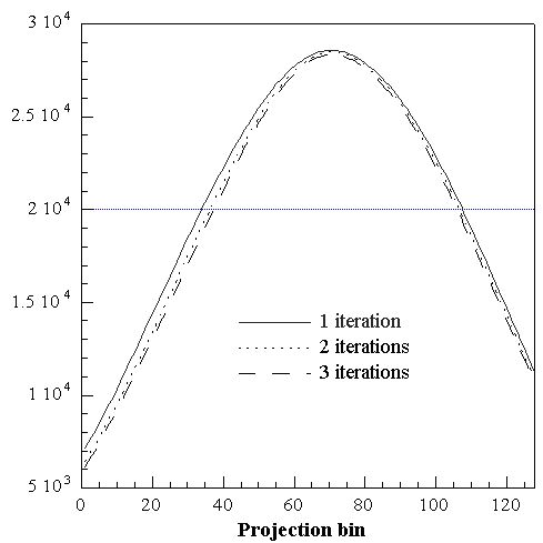 Fig. 7.16. : Profile of the scatter component in a projection plane of the clinical oncology study estimated by SRBSC with one (solid line), two (dotted line) and three full iterations (dashed line) of OSEM
7.6 Evaluation of scatter correction techniques
Scatter correction techniques can be evaluated using Monte Carlo simulation studies, experimental phantom measurements and clinical studies. Monte Carlo simulation is the gold standard since it allows to separate scattered and unscattered events and compare the estimated and true scatter components. Five scatter correction methods were compared in this section where applicable (Zaidi 2000b). The dual-energy window (DEW) technique, the convolution-subtraction method (CVS), two variants of the Monte Carlo-based scatter correction technique (MCBSC1 and MCBSC2) and statistical reconstruction-based scatter correction (SRBSC).
The DEW algorithm used is based on an implementation by the MRC PET methodology group at Hammersmith Hospital (UK) on the ECAT 953B scanner (Grootoonk et al 1996). The CVS method used is based on an implementation by Bailey and Meikle (1994). In this method, the scatter distribution is estimated by iteratively convolving the acquired projections with a mono-exponential scatter kernel. The scatter estimate is then subtracted from the measured data after scaling by an appropriate scatter fraction. The observed data are used as a first approximation to the unscattered distribution and the process is repeated iteratively with each step using the previous estimate of the scatter-free distribution as input to the scatter estimation. The number of iterations was four and the scatter fraction used was tailored to the phantom or clinical study under consideration. It ranges from 30% in 3D brain scanning to 45% in whole-body oncological studies. The other techniques were implemented according to the description provided in the preceding section.
7.6.1 Phantom simulation studies
Previously reported Monte Carlo validations of scatter correction techniques and related parameters have often been made by using simple source and attenuating medium geometries and compositions. In addition to these evaluations, there is also need to investigate more clinically realistic source distributions to validate and compare scatter correction techniques. A comparison of the relative performance of different methods are presented in this section using Monte Carlo simulated data of a digital brain phantom (Hoffman et al 1990). Evaluations have also been performed for the Utah phantom to characterise the differences between the methods for more standard geometries and allow determination of whether performance in the standard geometry predicts performance in the clinically realistic source distribution.
Different regions of interest (ROIs) were defined and the average number of events within each ROI computed for both ideal, non-corrected and scatter corrected images. With a few exceptions, most papers dealing with the evaluation of scatter correction techniques compare relative concentrations within different compartments of a given phantom with the background compartment serving as a reference. This approach is criticised because it and does not necessarily reflect the accuracy of the correction procedure and might bias the evaluation procedure. Hence, the evaluation reported here was performed in absolute terms. Contrast recovery can be viewed as an example of parameter estimation. It is defined as:
 |
(7.16) |
where NBG is the count density in the ROI corresponding to the background and Ncold is the count density in the ROI corresponding to the cold cylinder. Obviously, the ideal value is 100%. The activity recovery coefficients, defined as the percentage ratio of events in a ROI in the corrected images to events in the same ROI in the ideal images, were calculated according to:
 |
(7.17) |
where NROI is the count density in the ROI. The signal-to-noise ratio was defined as the mean number of events divided by the standard deviation of pixel intensities in a ROI defined within the background region A of the Utah phantom (Fig. 7.17).
 |
(7.18) |
7.6.1.1 The digital Utah multi-compartment phantom
Phantom simulations of the Utah multi-compartment phantom were carried out to assess the accuracy of scatter correction techniques. The compartments of the phantom were filled with relative concentrations in the different compartments of 1:2:0:2 in A, B, C and D, respectively (Fig. 7.17). In this study, the outer compartment (E), which is generally used to provide activity from outside the field-of-view was empty. ROIs with diameters approximately equal to half the radius of the small cylinders were placed in the various sections of the phantom and the mean counts/ROI in each section was determined.
 Fig. 7.17. : Diagram showing the different compartments of the Utah phantom used for quantitative analysis of the different correction techniques
The outer compartment (E) which is generally used to provide activity from outside the field-of-view is not shown.
The unscattered component in the simulated projection data was recorded and used as a reference to which the corrected projections using the different methods are compared. Fig. 7.18 shows a comparison of a profile through a sinogram plane representing the true unscattered component as estimated by the simulations and by the correction procedures. Most scatter correction techniques give a reasonable estimation of the scatter component and successfully bring the activity to zero faster outside the object.
 Fig. 7.18. : Integral profiles through a sinogram plane of unscattered events for the simulated Utah phantom and sinograms corrected using the different scatter correction techniques
For attenuation correction purposes, the determination of attenuation correction factors (ACFs) requires delineation of the object contour. One method of approximating the outline is by an ellipse. This method was applied in this study to determine the contour of the attenuating medium. A constant linear attenuation factor (m=0.096cm-1) was assumed for water. The 3D attenuation correction files are created by forward projection through the reconstructed 2D attenuation map. The reprojection method of Kinahan and Rogers (1989) was used to reconstruct the data sets. The maximum acceptance angle used for 3D reconstructions corresponds to a ring index difference of 11.
 Fig. 7.19. : Reconstructed images of the simulated Utah phantom
From top left, clockwise: the reference image used as input to the Monte Carlo simulations, reconstructed image of unscattered events only, NC, AC, CVS, SRBSC, MCBSC1 and MCBSC2.
The reference image, reconstructed image corresponding to unscattered events only and images reconstructed without applying any correction (NC), after correcting for attenuation alone (AC), and finally images obtained after applying scatter subtraction with different methods are illustrated in Fig. 7.19. All scatter correction techniques improve the quality of the images and allow a better definition of the cold cylinder (on the left) compared to the case where attenuation correction is applied alone, however, the images appear noisier when using Monte Carlo-based scatter correction. Horizontal profiles through the images shown in this figure are illustrated in Fig. 7.20.
 Fig. 7.20. : Horizontal profiles through the images shown in Fig. 7.19 illustrating : (a) the reference image used as input to the Monte Carlo simulations (solid line), reconstructed image of unscattered events only (dotted line), NC (small dashed line), AC (long dashed line) and (b) CVS (solid line), SRBSC (dotted line), MCBSC1 (long dashed line), and MCBSC2 (small dashed line)
Table 7.5 shows the estimated contrast and absolute concentrations in the different compartments of the simulated Utah phantom for one distribution of activity before and after 3D attenuation and scatter corrections are performed on the scans. An interesting observation from the analysis of the data presented in this table is that even in the reconstructed image corresponding to the unscattered component, the activity in the cold cylinder is not equal to zero as specified in the reference image used as input to the simulator. This difference may be attributed to detector scatter, the finite spatial resolution of the simulated scanner and partial volume effect. Scatter corrected images have poorer signal-to-noise ratio which can be explained by the scatter subtraction process and the resulting reduction in the statistics of the acquired data sets, however, the quantitative accuracy is greatly improved. A remarkable enhancement of the quantitative accuracy in the different compartments is noticed after scatter subtraction. The MCBSC2 method allows to obtain better contrast recovery in the cold compartment compared to the other methods at the expense of an increase in noise illustrated by a strong decrease of the signal-to-noise ratio. SRBSC slightly improves the SNR compared to the other techniques. While the quantitative accuracy of 3D PET is limited mainly by attenuation and scatter corrections, it may also be influenced by the choice of the reconstruction algorithm. It is important to know both systematic and statistical errors in activity quantification when using different reconstruction algorithms.
| Table 7.5. : Absolute concentrations and contrast measured in the different compartments of the simulated Utah phantom with and without attenuation correction and after applying the different scatter correction techniques |
| Figure of merit |
| Case/Compartment |
| Reference image |
| Unscattered image |
| AC |
| CVS |
| SRBSC |
| MCBSC1 |
| MCBSC2 |
The percent difference from true is shown in brackets. The signal-to-noise ratio (SNR) measured in the background is also shown. The outer compartment (E) was empty.
7.6.1.2 The digital Hoffman 3D brain phantom
In addition to standard source and phantom geometries, Eidolon uses integer matrices to simulate complicated and realistic source distributions. The mathematical source distribution of the Hoffman 3D brain phantom consists of 19 slices and is used to simulate a normal blood flow in the brain (Hoffman et al 1990). The specific activities of the grey matter, white matter and ventricles are 4:1:0, respectively. The original bitmaps were created in a 256x256 matrix size but were converted to 128x128 in our simulations.
The Hoffman 3D brain phantom was simulated and the results analysed as reported for the Utah phantom. The unscattered component in the simulated projection data was also recorded and used as a reference to which the corrected projections using the different methods are compared. Fig. 7.21 shows a comparison of a profile representing the true unscattered component as estimated by the simulations and the corrected data sets. Most scatter correction techniques overestimate the scatter component but successfully bring the activity to zero faster outside the object.
Reconstructions of the 3D digital Hoffman brain phantom without corrections, after applying attenuation correction alone and when using the different scatter correction algorithms are shown in Fig. 7.22. The low count regions and structures are better recovered after scatter compensation. The Hoffman brain simulation was evaluated by calculating the activity recovery for five circular ROIs over structures that are of special importance in neurophysiology. The image slice used for calculating the ROIs was the one including the basal ganglia and is illustrated in Fig. 7.23.
Table 7.6 shows the results of the quantitative evaluations of the percentage activity recovery using different correction techniques for the five circular ROIs which cover important structures of the brain. All scatter correction methods give very good activity recovery values for the simulated 3D Hoffman brain phantom which average within 3%. The CVS and MCBSC1 techniques tend to overcorrect while SRBSC undercorrects for scatter in most regions of this phantom.
 Fig. 7.21. : Integral profiles through the sinogram of unscattered events and sinograms corrected with the different correction techniques for the Hoffman 3D brain phantom
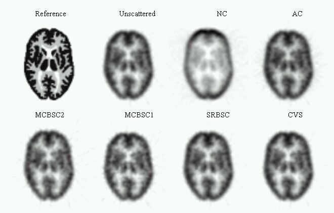 Fig. 7.22. : Reconstructed images of the simulated Hoffman 3D brain phantom
From top left, clockwise: the reference image used as input to the Monte Carlo simulations, reconstructed image of unscattered events only, NC, AC, CVS, SRBSC, MCBSC1 and MCBSC2.
 Fig. 7.23. : Digitised transverse slice through the basal ganglia chosen from the 3D Hoffman brain phantom indicating ROIs used in the quantitative evaluation of scatter correction methods
| Table 7.6. : Percentage recovery calculated in different structures of clinical interest in the Hoffman 3D brain phantom |
| |
| Structure |
| Frontal gyrus |
| White matter |
| CSF |
| Right thalamus |
| LMTG |
| Average |
| s.d. |
The average and standard deviation (s.d.) are also shown.
7.6.2 Experimental phantom studies
Experimental phantom studies were performed on the ECAT 953B scanner operated in 3D mode. Both the Hoffman 3D brain and Utah phantoms were scanned and analysed according to the same protocol used for the simulated data sets.
7.6.2.1 The physical Utah multi-compartment phantom
The Utah phantom was scanned with and without out of axial field-of-view activity. The outer compartment (E) was positioned just outside the FOV and contained no activity in the first acquisition, then it was filled with an activity concentration equal to that in the inner cylinder (background) for the second acquisition. The compartments of the phantom (Fig. 7.17) were filled with relative concentrations in the different compartments of 1:1.68:0:2.03 in A, B, C and D, respectively. ROIs with diameters approximately equal to half the radius of the small cylinders were placed in the various sections of the phantom and the mean counts/ROI in each section was determined. The reconstructed images of the physical Utah phantom without activity in the outer compartment are shown in Fig. 7.24. Horizontal profiles through the images shown in Fig. 7.24 are illustrated in Fig. 7.25.
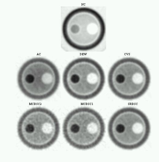 Fig. 7.24. : Reconstructed images of the physical Utah phantom without activity in the outer compartment (out of field-of-view activity)
The non-corrected image (NC) is shown for comparison purposes (top). The other images shown are from top left, clockwise: AC, DEW, CVS, SRBSC, MCBSC1 and MCBSC2.
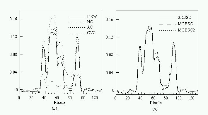 Fig. 7.25. : Horizontal profiles through the images shown in Fig. 7.24 illustrating : (a) NC (long dashed line), AC (dotted line), DEW (solid line), CVS (small dashed line), and (b) SRBSC (solid line), MCBSC1 (small dashed line), and MCBSC2 (dotted line)
The results of the quantitative analysis of the data are summarised in table 7.7. All the methods improve the contrast compared to the case where no correction is applied. All the methods improve the contrast compared to the case where no correction is applied. It can be seen that the DEW method predicts the contrast very accurately as compared to the other methods but increases the noise significantly. On the other hand, SRBSC has better SNR and gives good contrast and quantitative accuracy in the outer compartment.
| Table 7.7. : Absolute concentrations and contrast measured in the different compartments of the scanned Utah phantom with and without attenuation correction and after applying the different scatter correction techniques |
| Figure of merit |
Absolute concentration (kBq/ml) |
Contrast (%) |
SNR |
| Case/Compartment |
B |
D |
C |
A |
| Calibration concentration |
5.88 |
4.86 |
100 |
- |
| AC |
7.66±0.28 |
5.31±0.17 |
63.82±1.15 |
21.91±5.17 |
| DEW |
6.05±0.23 |
4.62±0.18 |
91.63±1.84 |
15.42±3.64 |
| CVS |
6.49±0.30 |
4.68±0.23 |
84.11±3.85 |
18.79±4.54 |
| SRBSC |
6.52±0.30 |
4.76±0.22 |
86.26±3.95 |
19.46±4.72 |
| MCBSC1 |
6.51±0.24 |
4.81±0.21 |
81.31±3.93 |
9.74±2.43 |
| MCBSC2 |
6.55±0.27 |
4.78±0.15 |
85.02±1.76 |
10.32±2.05 |
The percent difference from true is shown in brackets. The signal-to-noise ratio (SNR) measured in the background is also shown. The outer compartment (E) was empty.
The Utah phantom was then scanned with out of field-of-view activity. The outer compartment (E) was positioned just outside the FOV and contained an activity concentration equal to that in the inner cylinder (background). The data sets were analysed as before. Fig. 7.26 illustrates the reconstructed images of the Utah phantom with activity in the outer compartment. Horizontal profiles through the images shown in Fig. 7.26 are illustrated in Fig. 7.27.
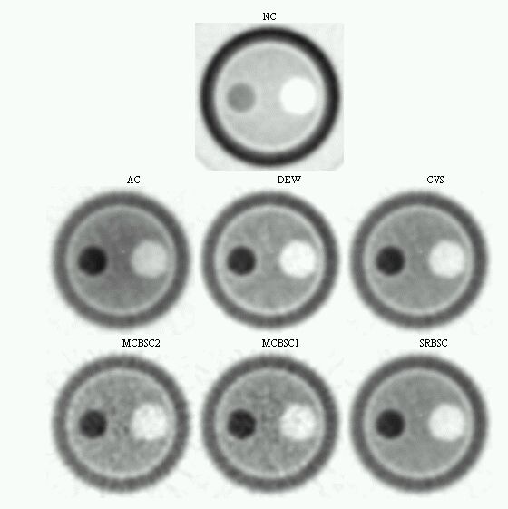 Fig. 7.26. : Reconstructed images of the physical Utah phantom with activity in the outer compartment (out of field-of-view activity)
The non-corrected image (NC) is shown for comparison purposes (top). The other images shown are from top left, clockwise: AC, DEW, CVS, SRBSC, MCBSC1 and MCBSC2.
The results of the quantitative analysis of the data are summarised in table 7.8. Again the DEW predicts the contrast very accurately as compared to the other methods. Statistical noise was insignificantly changed by CVS and SRBSC whereas it was increased slightly by DEW and significantly by Monte Carlo-based approaches. The DEW method was more successful in correcting for scatter originating from outside the FOV. This was expected and already reported by other groups (Townsend et al 1996) since the CVS and SRBSC techniques estimate the scatter directly from measured data whereas the DEW method is sensitive to contributions from both in- and out-of FOV activity.
 Fig. 7.27. : Horizontal profiles through the centre of the images shown in Fig. 7.26 illustrating : (a) NC (long dashed line), AC (dotted line), DEW (solid line), CVS (small dashed line), and (b) SRBSC (solid line), MCBSC1 (small dashed line), and MCBSC2 (dotted line)
| Table 7.8. : Absolute concentrations and contrast measured in the different compartments of the scanned Utah phantom with and without attenuation correction and after applying the different scatter correction techniques |
| Figure of merit |
Absolute concentration (kBq/ml) |
Contrast (%) |
SNR |
| Case/Compartment |
B |
D |
C |
A |
| Calibration concentration |
5.88 |
4.86 |
100 |
- |
| AC |
7.94±0.30 |
5.47±0.15 |
64.60±1.08 |
19.04±4.69 |
| DEW |
6.14±0.21 |
4.61±0.10 |
95.74±2.09 |
12.37±3.97 |
| CVS |
6.72±0.32 |
4.82±0.20 |
84.90±3.34 |
16.24±4.33 |
| SRBSC |
6.76±0.32 |
4.90±0.19 |
86.78±3.30 |
16.81±4.60 |
| MCBSC1 |
6.62±0.31 |
4.72±0.24 |
86.23±2.64 |
9.78±3.37 |
| MCBSC2 |
6.77±0.24 |
4.94±0.18 |
86.33±1.54 |
9.33±2.33 |
The signal-to-noise ratio (SNR) measured in the background region is also shown. The outer compartment (E) was filled with an activity concentration equal to that in the background region.
7.6.2.2 The physical Hoffman 3D brain phantom
A physical Hoffman 3D brain phantom with a grey-to-white matter ratio of 5:1 (Hoffman et al 1990) was filled with 18F taking care to avoid introducing air bubbles. The data were acquired with moderate statistics (40 Mcounts). The reconstructed images without and with the different correction techniques are shown in Fig. 7.28. It is hard to judge any major differences in the corrected images. The effect of scatter removal in areas where no activity is present is, however, clearly seen (e.g. CSF). The DEW method slightly improves the contrast compared to the other methods.
 Fig. 7.28. : Reconstructed images of the physical Hoffman 3D brain phantom
The non-corrected image (NC) is shown for comparison purposes (top). The other images shown are from top left, clockwise: AC, DEW, CVS, SRBSC, MCBSC1 and MCBSC2.
7.6.3 Clinical studies
The different scatter correction algorithms were also tested on clinical data obtained on the PRT-1 scanner from the Geneva University Hospital (Townsend et al 1993). A cerebral and whole-body clinical study were selected from the database and used for clinical evaluation of the scatter correction methods.
7.6.3.1 Brain scan study
A clinical brain scan of a patient who was referred to the Nuclear Medicine Division of Geneva University Hospital for evaluation was studied. A transmission measurement (15 min) using 68Ge rotating rod sources was performed for attenuation correction purposes. The emission study started 30 min after intravenous injection of 18F-FDG. The study was reconstructed by 3DRP with and without applying attenuation and scatter correction techniques. Fig. 7.29 displays an image plane from the uncorrected, attenuation corrected and scatter corrected brain study. Again, it is hard to judge any major differences in the corrected images. Nevertheless, the corrected images have poorer signal-to-noise ratio but better overall contrast than the uncorrected original image.
Scatter correction improves the contrast between grey and white matter. An analysis of the difference images between non-corrected and scatter corrected data (not shown) revealed the regional effect of scatter correction on the data. In particular they look like attenuation corrected images, especially the contrast between the brain tissue and the air filled sinuses. Results obtained using the CVS approach for scatter correction in cerebral 3D PET scans (homogeneous attenuating region) have proven to be accurate (Bailey and Meikle 1994). Similar performances are obtained with our newly developed SRBSC approach which is well adapted to this kind of studies.
 Fig. 7.29. : Reconstructed images of a clinical brain study: from top left, clockwise: NC, AC, CVS, SRBSC, MCBSC1 and MCBSC2
7.6.3.2 Clinical oncology study
An oncology study issued for a woman with a known stage T4 neoplasm of the breast and two metastases in the lung and the mediastinum was also considered. Data acquisition was performed at four bed positions covering an axial field-of-view of approximately 35 cm (4 volumes, 15 min/volume) Transmission measurements were performed at each bed position (10 min/position). The Monte Carlo package performs in principle a simulated 3D PET acquisition of a single bed position of the scanner axially positioned over the lungs and heart. Out-of-FOV activity was also incorporated by including 3 bed positions one below and 2 above the simulation FOV. The study was reconstructed by 3DRP with and without applying the different correction techniques.
Fig. 7.30 illustrates a slice from the uncorrected and scatter corrected 3D clinical study at the level of the thorax. It should be noted that for the whole-body, it is difficult to assess the effect of the scatter correction in the images shown. However, the streak artefacts seen in the attenuation corrected image only have been reduced after scatter subtraction by all techniques.
The physics of photon interactions indicates that in a low density region, the amount of scattering is negligible. However, many incorrectly positioned LORs will be assigned to projection data through the low density region with similar probabilities to an adjacent, more dense region, as a result of the coincidence detection method (Bendriem and Townsend 1998). This is a possible explanation for the fact that the presence of a small, low density region will hardly be visible on the scatter profile in the projection data. However, for obvious reasons, the measured attenuation correction factors applied to this low density region will be lower. The resulting effect after reconstruction is the underestimation of scatter contribution from this region. This illustrates one of the possible interactions of scatter correction with the other correction and processing techniques (e.g. attenuation).
 Fig. 7.30. : Reconstructed images of an oncology study at the level of the thorax. From top left, clockwise: NC, AC, CVS, SRBSC, MCBSC1 and MCBSC2
It has been shown in this chapter that the parametrization of the scatter response function can be obtained by Monte Carlo simulations and that the inherent assumptions in convolution-subtraction based approaches are still valid even in large objects like the thorax of a patient. Both CVS and SRBSC scatter correction approaches use a constant scatter response function and a global scatter fraction estimated from scanning standard objects equivalent to the size and shape of patients (in this case a line source in a uniform water-filled cylinder).
It is believed that an accurate estimation of the scatter fraction is more important than modelling the spatially-variant scatter functions (Bendriem and Townsend 1998). The results presented in this chapter seem to confirm this statement and suggest that these correction techniques are applicable to both cerebral 3D PET scans and more heterogeneously attenuating regions of the body such as the thorax. Nevertheless, the nonstationary assumption overcomes the inherent limitations of the stationary approach by taking into consideration the dependence of scatter upon source locations, object size, detector angle, etc. Different methods of nonstationary deconvolution have been proposed in the literature (Ljungberg and Strand 1990, Welch et al 1995). Such an approach is further discussed in future developments section of chapter 8, where a new method under development is described. The neural networks approach for scattered photons discrimination has also been reported by other research groups (Ogawa and Nishizaki 1993).
This chapter has focused mainly on the use of Monte Carlo simulations to study scatter associated with 3D PET imaging. Because of the finite energy resolution of block detectors, discrimination between unscattered and scattered events is not an easy task. Most experimental investigations of scatter have been limited to simple homogeneous and symmetric phantoms. The development of efficient Monte Carlo simulation packages has allowed the study of scatter for realistic distributions and attenuation maps and according to a variety of physical parameters. Monte Carlo studies have been used to study the spatial characteristics of scatter versus energy. In addition, the Monte Carlo method is uniquely able to provide information about multiple- versus single-scatter events. Knowledge gained from Monte Carlo simulations has contributed to the formulation and evaluation of new scatter correction techniques in 3D PET.
In summary, the quantitative accuracy and noise characteristics of different types of scatter correction techniques were investigated with both simulations, phantom measurements and clinical studies. All correction methods significantly improved the image contrast. Generally, it was shown that the differences in the estimated scatter distributions did not have a significant impact on the final quantitative results. Detector scatter leads to a slight blurring of the intrinsic spatial resolution of a tomograph, however, for current-generation commercial PET systems, this contribution is minimal.
In this study, the DEW method was found to be clearly superior in the experimental phantom studies in terms of quantitative accuracy at the expense of a significant deterioration of the SNR. On the other hand, the immunity to noise in emission data of statistical reconstruction-based scatter correction methods make them particularly applicable to low-count emission studies. The DEW method is the easiest method to implement, but requires a system-specific calibration. A major disadvantage is that some commercial systems do not allow acquisition of coincidence events in separate windows (e.g. GE-Advance).
Contribution of scatter from outside the FOV is a challenging issue that needs to be addressed with large axial FOV 3D PET scanners. Townsend et al (1996) investigated the effect of scatter from outside the FOV on the quantitative accuracy of parameter estimations in brain studies using 11C-Flumazenil tracer. The same conclusions reported by us were drawn based on phantom studies regarding the performance of the DEW approach for scatter correction as compared to the CVS technique. Nevertheless, the authors claim that this is not a major problem in cerebral studies and small axial FOV tomographs. The problem remains crucial for abdominal and thoracic studies where contribution of scatter from outside the FOV is not negligible. Further evaluation of the algorithms using simulated clinically realistic distributions in non-uniform attenuating regions like the thorax (e.g. Zubal phantom) is still required.
The Monte Carlo-based scatter correction procedure may be repeated iteratively to reduce systematic errors introduced by the presence of scatter in the input images and the low statistics in the simulated data. It is well recognised that Monte Carlo-based scatter correction may not be practical for clinical routine applications with common computing facilities available in PET centres. However, powerful multiple-processor parallel processing systems are becoming more accessible to the scientific community, therefore investigation and characterisation of such correction techniques and the effect of different approximations on their accuracy is worthwhile. We believe the basic principles of the method could also be applied to other scanner geometries including the combined PET/CT system and to other imaging modalities such as transmission CT and SPECT. However, the success of such applications will depend on the efficient and accurate calculation of scatter responses from objects with non-uniform density and on the availability of suitable Monte Carlo simulators.
The SRBSC approach is computationally efficient as it can be easily implemented on vector or parallel computing hardware and the software required either for forward projection or fast Fourier transform is widely available in the public domain. Moreover, the low spatial frequency nature of the scatter distribution allows to reduce the data size by coarse rebinning in the radial and axial direction without sacrificing the accuracy in the scatter distribution estimation.
For iterative-based scatter compensation, there are some simple ways in which the amount of computation time can be reduced. For example, the scatter distribution may have to be re-calculated a few times only, since the calculated scatter estimate does not change much after only a few iterations of accelerated reconstruction algorithms like OSEM. The scatter estimate can be kept as a constant term in later iterations instead of modifying the scatter estimate in each iteration (Hutton and Baccarne 1998). Alternatively, it may be worth investigating whether it is adequate to only approximate scatter modelling in the first couple of iterations, and re-calculate the scatter distributions only for latest iterations.
8. Concluding Remarks and Future Work
In many respects, the field of nuclear medicine has been ahead of other areas of image science in objective assessment and optimisation of image quality. Nuclear medicine has poor spatial resolution compared to other imaging modalities in radiology, although its ability to measure physiological processes is unsurpassed. While the potential for PET in this field is undisputed, the challenges must also be recognised. PET is a spin-off from medical physics which has today an important clinical impact in neurology, oncology and cardiology. The Geneva University Hospital has already ordered a 18 MeV cyclotron and is currently setting up a production facility for positron emitting radiopharmaceuticals. The PET centre in the Geneva region is expected to be a unique opportunity and a significant step forward for Swiss neuroscience and oncology researchers.
When the partners of the PARAPET project started to write the proposal to the European Commission, they decided to include a full workpackage devoted to the development of Monte Carlo simulators for both cylindrical and dual-head PET tomograph geometries and a second one for the generation of data sets to be used for both testing the algorithms during the development stage and the comparative evaluation of reconstruction techniques. The main motivation was to use the simulators to generate data sets in a controllable manner and to assess the effect of different parameters on the images reconstructed by different techniques. The Parsytec CC high performance parallel platform available to us through this project allowed us to further work on portability issues of the software and to generate the data in an acceptable time compared to a single-processor system.
In conclusion, let us review what concrete results have been achieved through the developments presented in this thesis, what the implications of this work are in a clinical and research environment, and which directions of future research work arise as its logical consequence.
8.1 Key conclusions
Monte Carlo modelling has contributed to a better understanding of the physics of photon transport in medical physics. The large number of applications of the Monte Carlo method attests to its usefulness as a research tool in different areas of nuclear medicine imaging including detector modelling and systems design, image reconstruction and scatter correction techniques, internal dosimetry and pharmacokinetic modelling. Monte Carlo simulation is a gold standard for the simulation of PET data and is an indispensable research tool to develop and evaluate scatter models. The recent interest in the development of high-resolution PET scanners and multiple-processor parallel processing systems has created new opportunities for Monte Carlo simulation in PET imaging (Zaidi 1999a).
Modelling of imaging and other medical applications is best done with phantom models that match the gross parameters of an individual patient. Recent three- and four-dimensional computer phantoms seek a compromise between ease of use, flexibility and accurate modelling of populations of patient anatomies, and attenuation and scatter properties and biodistributions of radiopharmaceuticals in the patients. Current developments are aimed at computer phantoms that are flexible while providing accurate modelling of patients. Modelling of the nuclear medicine imaging process has been improved by more accurate simulation of the physics and instrumentation involved in the process. Monte Carlo software packages, especially those developed specifically for nuclear medicine and with different performance characteristics, have been found useful in the modelling work. A major limitation has been the long simulation time required by the intensive computations. With advances of computer technologies and implementation techniques, we are able to model interactions of radiation within the patient and characteristics of the imaging system with much improved accuracy in an increasingly shorter computational time. The combination of realistic computer phantoms and accurate models of the imaging process allows simulation of nuclear medicine data that are ever closer to actual patient data. Simulation techniques will find an increasingly important role in the future of nuclear medicine in light of further development of realistic computer phantoms, accurate modelling of projection data and computer hardware. However, cautions must be taken to avoid errors in the simulation process and verification via comparison with experimental and patient data is essential.
The image quality of PET reconstructions is degraded by a number of physical factors including: (i) the attenuation of the photons travelling towards the detector; (ii) the detection of scattered as well as primary photons; (iii) the finite spatial resolution of the imaging systems; (iv) the limited number of counts one is able to collect when imaging patients; and (v) physiological as well as patient motion. Historically, once one had obtained the best projection data feasible, one typically applied compensations for these degradations either prior to or after reconstruction with filtered back-projection. Currently, the preferred compensation strategy is becoming the incorporation of modelling these degradations into an iterative reconstruction method. This trend is likely to continue into the future, and these methods become routinely employed clinically. It has been shown that iterative methods drastically improve the quality and quantitative accuracy of PET images. The benefits of developing a flexible, modular and parallel 3D reconstruction library within the PARAPET project are now becoming clear. According to our and other partners' experience, implementation of existing and new reconstruction techniques can be done in an efficient way.
To perform scatter compensation one has to estimate the contribution of scatter to the images. Typically the methods for doing this have been based on either energy spectrum or spatial response approaches. Energy spectrum methods involve the acquisition of anywhere from one additional window below the photopeak window to that of the entire energy spectrum for each pixel. This data can be interpolated (extrapolated) in any number of ways to provide a pixel specific scatter estimate. Spatial domain methods apply scatter models in combination with the emission data and possibly estimates of the attenuation map to estimate the contribution of scatter. Once the estimate is obtained, it can be subtracted from the projection data, or used and updated as part of iterative reconstruction. Fairly exact modelling in iterative reconstruction may become the method of choice as computing times and algorithms continue to improve.
An improvement and extension to whole-body 3D imaging of a recently proposed Monte Carlo-based scatter correction (MCBSC1) method has been presented in this thesis (MCBSC2). A new scatter correction method called Statistical Reconstruction Based Scatter Correction (SRBSC) based on estimating the low frequency component corresponding to scatter events using OSEM is also proposed and evaluated against more common correction methods. Five scatter correction methods based on subtracting an estimated scatter component from the projection data have been compared where applicable. The dual-energy window (DEW) technique, convolution-subtraction method (CVS), two variants of the Monte Carlo-based scatter correction technique (MCBSC1 and MCBSC2), and SRBSC. The aim was to compare the estimated scatter distributions with the true scatter distribution in the photopeak window. It has been shown that parametrization of the scatter response functions can be obtained by Monte Carlo simulations and that the inherent assumptions in convolution-subtraction based approaches are still valid even in large objects like the thorax of a patient. The statistical errors in the scatter corrected data have not been fully investigated. The error propagation has not been fully analysed and therefore no error limits have been given. In order to fully compare the scatter correction methods, further evaluation of the uncertainty in each correction needs to be made. It was concluded that all the methods improve the contrast compared to the case when no correction is applied and that an accurate modelling of the scatter component is essential for a proper scatter correction.
It might also be possible to combine the currently implemented variance reduction with other variance reduction methods (see Zaidi 1999a for an overview of variance reduction techniques which have been applied to the Monte Carlo simulation of emission tomography). However, as processors become faster and the number of processors per computer increases, the method should soon become practical for routine scatter correction, even without adding any of the possible acceleration methods. Together with the optimisation of the computing time performances of the Monte Carlo software, photon transport in 3D PET could be efficiently modelled to better understand scatter correction techniques. The accuracy in correction methods can thus be evaluated in an unbiased way since systematic errors can be controlled. The improved accuracy and speed-up due to parallelisation makes Monte Carlo simulation more attractive as a tool for modelling photon transport in 3D PET.
8.2 Future aspects of quantitative 3D PET
Positron emission tomograph design has an interesting history. It includes early systems based on gamma cameras, the use of discrete detectors in opposing planar arrays as well as rings, the use of a variety of scintillators (e.g. NaI(Tl), BGO, BaF2, plastic, LSO), and systems based on wire chambers and hybrids of wire chambers and scintillators. As we head into the year 2000, we have seen some of the old technologies used in PET systems re-emerge (e.g. dual-head gamma cameras operated in coincidence mode) as well as new scintillators and new detector design directions (e.g. layered crystals with pulse-shape discrimination). Wire chambers of various kinds are also still being developed for PET applications. Phoswich detectors are also receiving considerable attention for the design of dual-modality scanners (PET/SPECT). As PET has become of more interest for clinical practice, several different design trends seem to have developed. Systems are being designed for 'low-cost' clinical applications, very high resolution research applications, and just about everywhere in-between.
All of these systems are undergoing revisions in both hardware and software components. New technologies that are emerging include the use of LSO and GSO as alternatives to BGO crystals, the use of layered crystals and other schemes for depth-of-interaction determination (for dedicated systems) and for hybrid SPECT/PET devices (e.g. NaI(Tl)/LSO). In addition, high resolution animal scanner designs are plentiful and one such device is now being offered commercially. Thus, there are many different design paths being pursued - which ones are likely to be the main stream of future commercial systems? The SPECT/PET systems are pushing ahead for higher count rate performance (still a major area of difference between hybrid and dedicated PET systems) and effective scatter and attenuation correction capabilities. The dedicated systems seem to be splitting into two major design paths: (i) lower cost yet higher performance whole body imaging systems; and (ii) very high spatial resolution systems aimed primarily at research applications. The major technologies currently under development seem to be centred around improved, cheaper electronics and better scintillators. One technology that has yet to make a large impact in this field is the use of solid state devices - either for light collection or primary photon collection. The problem has usually been cost, but new technology may yet allow such devices to be considered for future PET systems. It will be interesting, indeed, to see what technologies become the most popular in the future.
Modern image reconstruction methods involve two key components. The 'software' of image reconstruction is an objective function (e.g. the likelihood function) that describes the acceptability of an image solution. The 'hardware' is the algorithm for optimising the objective function to find the best solution. In recent years, 'hardware' components such as the OSEM algorithm, have been widely studied with an aim toward producing image reconstruction algorithms that will be practical in the near term. With advances in computer technology (e.g. multiprocessor PCs and PC clusters) and optimisation techniques (e.g. Monte Carlo Markov Chain methods), the machinery of optimisation will allow more complex objective functions to be used; thus, the 'software' of image reconstruction will become the dominant open issue. The research community's relative lack of success in developing good Bayesian priors for image reconstruction is one explanation. Simple priors, or no priors at all, have often been preferred to sophisticated edge-preserving priors that tend to create unnatural image results.
The feasibility of using the IMC procedure for image reconstruction in 3D PET needs to be explored and validated. Much work remains to fully refine and evaluate the IMC technique (see chapter 3) as a clinically viable reconstruction algorithm for 3D PET. While theoretically pleasing, the EM algorithm is only one way to solve the problem. Some combination of alternative statistical or algebraic reconstruction techniques utilising the accurate system modelling provided by Monte Carlo, will hopefully result in a reconstruction algorithm for PET with simultaneous compensation for attenuation and scatter which is versatile and rapid enough for routine clinical use. The preliminary results obtained so far demonstrate that the development of IMC is a major step toward the realisation of quantitative PET. Some of the parameters of the IMC algorithm that need to be optimised are the choice of the first source estimate, the number of iterations or the stopping criteria and the lowest acceptable number of events to simulate per iteration for the forward projection step. Increasing the number of simulated events reduces statistical fluctuations of the simulated data and yields better images but increases the reconstruction time. There are various choices for the first estimate of the source distribution, such as uniform field, or an image obtained from earlier iterations or another reconstruction algorithm such as FBP. Some groups reported that the use of the backprojection of the measured data as the first estimate is a good starting point (Kudrolli et al 1999).
Within the already mentioned PARAPET project, an extensive evaluation of iterative vs. analytical algorithms will be performed and the improvement in image quality and quantitative accuracy resulting from the use of iterative techniques will be investigated. General purpose comparative evaluation of different methods for 3D PET reconstruction is inherently difficult due to the multiplicity of the medical purposes for which the reconstructions may be studied (Furuie et al 1994). For any specific medical task, the evaluation should ideally be based on the performance of human observers (Swets and Pickett 1982). However, this is costly and complex, since a number of observers should be used, each has to analyse many images, conditions have to be carefully controlled, and so on.
Completion of the proposed SRBSC algorithm for scatter correction by including accurate models for detector efficiency, multiple scatters, scatter from outside the field-of-view and a number of minor improvements would enable quantitative, fully 3D PET imaging in the head and the body. This would affect specific protocols in one of two ways. Protocols for which counting statistics are adequate can be run in 3D with less than one-third the patient dose, thereby improving the safety of the method. In other protocols, such as FDG cancer imaging where sensitivity is important, the image variance can be reduced by a factor of three to four. This would significantly improve the statistical power of conclusions drawn from research studies, improve diagnostic accuracy, and reduce the number of data sets discarded because of poor counting statistics.
Another approach to Monte Carlo-based scatter correction would be to extend the technique originally proposed for SPECT by Ljungberg and Strand (1990) to 3D PET. In this technique, Monte Carlo simulated scatter fractions and scatter line-spread functions (SLSF) for different depth and lateral positions are used. A reconstructed emission image is used as an estimate of the source distribution in order to calculate the scatter contribution in the projection data. Correction for non-uniform scatter is made by a convolution technique based on the calculated SLSF. The scatter contribution is then subtracted from the original projection prior to attenuation correction. The calculation of scatter fractions and scatter function distributions have already been made using our Monte Carlo software in uniform attenuating medium which would facilitate the implementation of the method in clinical cerebral 3D PET imaging. Further validation in clinically realistic distributions and non-uniform attenuating regions like the thorax need to be performed.


 such that

 1 for x in [xmin, xmax],
 as the pdf,
 , i.e. choose a random number R, if
  , accept x, otherwise go back to step (iii).


 .
.

 (Moses et al 1998), where d is the detector size and b is a factor due to the crystal decoding process (0 if the crystal of interaction is individually coupled to a photodetector and approximately 2.2 mm otherwise). This factor while empirically determined for BGO detector modules, has been found to be necessary to 'predict' the performance of several new high-resolution PET cameras (Moses et al 1998). The same paper suggests an empirical formula for calculating the linear fluctuations due to photons non-collinearity in any given direction which can be modelled as a Gaussian distribution (around 180° with an FWHM of about 0.3°) centred at the origin and expressed as snon-col = 0.0022 x Ds, where Ds is the scanner's diameter (in mm). The intrinsic spatial resolution calculation for the ECAT 953B scanner when using 18F is estimated as 3.96 mm according to:


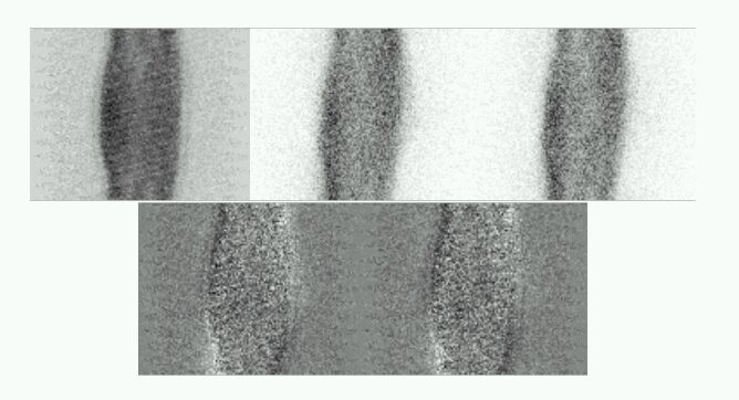


 .
.


 are directly available for individual elements, the linear attenuation coefficients for mixtures and compounds are obtained according to:
 values at every absorption edge for all constituent elements, interpolation was performed separately for the cross sections indicated in Eq. (6.2), including the photoeffect cross sections for the individual atomic subshells. This program was used to calculate the attenuation coefficients for the selected compounds presented in this section.
 . The photoelectric total cross section per atom have been parameterized as:
 .
.


 . The fit was made over 511 data points chosen between
 .
.
 , where mc is the coefficient being compared and mEPDL97 are the EPDL97 coefficients. The comparisons shown in Fig. 6.6 and Fig. 6.7 are continuous and were calculated at 1 keV intervals between 1 and 1000 keV for both XCOM and PHOTX, between 10 and 1000 keV for GEANT, and between 15 and 511 keV for PETSIM. It can be seen that the differences can be as large as 20%. For PHOTX, the strong variations and oscillations visible in the plots as high frequency quasiperiodic noise is thought to be due to the discrete nature of the source data and the crude interpolation used between the known coefficients which was chosen mainly to mimic the standard method used by most Monte Carlo developers.