As an example we consider here the relationship between left right self-placement and support for Switzerland being a member of the European Union.

If we consider the marginal frequency of this table, it appears that 58% of the sample is in favour of EU membership. If left-right self-placement were totally independent from support for European integration, one would expect 58% of the leftists, 58% of centrists and again 58% of the right-wingers to be in favour of Switzerland's membership of European Union. This is obviously not the case, but as we are working with random samples we must first assume that the actual difference between, for example left and centre of 15.7%, is just random, i.e. due to sample fluctuations. Before interpreting the differences and the relationship we are assuming that the variables are and have to ask first, whether the relationship is .

Let us work out this assumption of independence (the independence model). Very precisely, the probability to be in favour of EU integration is 57.98% (414/714), the probability to be left is 24.09% (172/714). So if the two variables were totally independent we would expect roughly 100 leftists to be in favour of European Union membership =(0.5798*0.2409*714). This frequency is called the . As we can see, the in this cell is 130 (the leftists in favour of EU membership in our sample). This means that we have roughly 30 more than expected. This value is the difference between the observed and expected frequency (difference from independence).

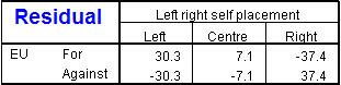These differences (also called "residuals") from the independence table (table of expected frequencies) are the basis of the statistic.

Crosstabs lets you produce tables containing observed, expected and residual (unstandardized) frequencies. (Select from the Cells dialog or use syntax.
CROSSTABS /TABLES=q28r BY d01r /CELLS= COUNT EXPECTED RESID .

The χ² statistic is based on the difference between the expected and the observed number of cases and it permits to test the hypothesis that row and column variables are independent.

It is calculated by summing over all cells the squared residuals divided by the expected frequency.

In our case the χ² value, as we can see under "Pearson chi-square" in the output, is:

54.28 = (30.3)²/99.7 + (7.1)²/209.9 + (-37.4)²/104.4+
      (-30.3)²/72.3 + (-7.1)²/152.1 + (37.4)²/75.6

Generally a statistical test works as follows: Your research hypothesis is that there is a relationship between self-placement on the left-right scale (3 categories) and EU membership; when looking at our table we want to know whether we can interpret the relationship we see in the table (based on a random ), as a relationship among all Swiss citizens (), i.e. in other words can we from the sample that there is a "true" relationship in the population. ()

• Formulate a that the two variables are and a that the variables are dependent. More precisely statistical testing is about finding out whether we can reject the [H₀] (and therefore accept the [H₁] or if we have to keep H₀.
• Specify significance level (α) that defines a threshold, indicating what risk you are prepared to take when deciding. In statistics certainty does not exist, we will never be sure, there is always a probability that the be true, but we want that probability to be low, how low is indicated by that level. Typical levels considered are 0.05 (or 5%), 0.01 (or 1%), 0.001 (1‰). Never forget that choosing a level is your personal decision stating the risk you are prepared to take that H₀ is true when you decide to reject it. To make it very clear: In a medical experiment with a possible lethal issue for your patients, would you accept an α level of 0.05 that it implies a risk of 5 patients out of 100 dying because of your experiment?
• Compute a test statistic (χ² statistic)from the table and compare it to the theoretical χ² distribution.
• If the probability that the relationship could have been produced by chance (this is same as saying the is true) is below the threshold we have set (), we reject the : this implies accepting the in order words we can say the variables are dependent (related).

To perform the χ² test, we will have to compare the calculated χ² statistic to the critical points of the theoretical χ² distribution. To do that SPSS computes the probability that the observed χ² could have been produced by chance (just random fluctuation).

More specifically, on the SPSS output you will find under Asymp. Sig. (2-sided) a value of 0.000. As this value (probability), often called the , is lower than the (threshold) you have specified, let's say 0.01, we can reject the .

Above we have explained the classical χ² statistic, also called the Pearson χ². There are other, for example the ("Likelihood ratio" in the output) is an alternative to the . It is based on maximum-likelihood theory. For large samples it is identical to Pearson χ². It is recommended especially for small samples.

The magnitude of the χ² statistics depends not only on goodness of fit, but also on the sample size. If the sample size is multiplied by n, so does the χ² statistic. This means that for large sample sizes, nearly every relationship is statistically significant, small samples nearly never are. For these reasons, one must be very cautious about the interpretation, as statistical significance is related to sample size.

The expected frequencies for each category should be at least 1.

No more than 20% of the categories should have expected frequencies of less than 5. This can happen for small samples or crosstabulations with many cells. SPSS supplies this information in a note at the bottom of the "Chi-Square Tests" table.

On the table you will also fined a column labelled "df". This corresponds to the . As the chi-square test depends also on the number of rows and columns of the table. For a r x c table it is (r-1) x (c-1). Our table here, as you can see in the output has 2 degrees of freedom ("df" on the same line) which is simply (2-1) x (3-1). The degrees of freedom can be viewed as the number of cells that need to be set, until all others are fixed, given the constraints of the marginal frequencies.

Note as SPSS supplies the actual p-value, there is no need to look up the chi-square statistic's value in a statistical table printed in a book and find there the critical value corresponding to both the and the .